Statistics

6.1. INTRODUCTION
We have studied in previous class about the classification of given data into ungrouped as well as grouped frequency distributions. We have also learned how to represent the data with the help of various graphs like bar graphs, histograms, and frequency polygons. Now, we will study certain numerical representatives of the ungrouped data, mean, median, and mode. In this chapter, we will study mean, median, and mode from ungrouped data to that of grouped data. Besides this, we will know the concept of cumulative frequency, the cumulative frequency distribution, and also how to draw cumulative frequency curves.

6.2 MEAN OF GROUPED DATA
The mean (or average) of observations is the sum of the values of all the observations dived by total number of observations. If $x_1, x_2, x_3 ...... x_n$ are observation and their respectively frequencies are $f_1, f_2, f_3, ...... f_n$, then this mean observation $x_1$ occurs $f_1$ times, $x_2$ occurs $f_2$ times, and so on.
Then, the sum of the values of all observations = $f_1{x}_1+f_2{x}_2+f_3{x}_3+.......+f_n{x}_n$  and the sum of number of observations = $f_1+f_2+f_3+......+f_n$ .
Hence, the mean  of the data is represented by
$\overline{x} =\frac{f_1{x}_1+f_2{x}_2+f_3{x}_3+.......+f_n{x}_n}{f_1+f_2+f_3+.......+f_n}$

So,     $\boxed{\overline{x} =\frac{\sum f_i{x}_i}{\sum f_i}}$       …. (i)

[Where $\sum$ means summation and i means 1 to n.]

Assumed Mean Method
We choose assumed mean a (say) and subtract if from each of the values $x_i$. The reduced value
$x_i$ – a is called the deviation of $x_i$ from a. The deviation are multiplied by corresponding frequencies to get $f_i{d}_i$. On adding all $f_i{d}_i$ we get the sum, i.e. $\sum f_i{d}_i$ .
Let $x_1, x_2, x_3, ..... x_n$ be values of a variable x, with corresponding frequencies $f_1, f_2, f_3, .... f_n$ respectively.
di = $x_i$ – a;         
where i = 1, 2, 3, … n
$\Rightarrow f_i{d}_i =f_i(x_i–a)$  ;    where i = 1, 2,3, … n

$$\begin{gathered} \Rightarrow \sum f_i{d}_i = \sum f_i(x_i–a) \\ \Rightarrow \sum f_i{d}_i =\sum f_i{x}_i–a\sum f_i \end{gathered}$$

on dividing by $\sum f_i$ , we get

$$\begin{gathered} \frac{\sum f_i{d}_i}{\sum f_i} =\frac{\sum f_i{x}_i}{\sum f_i}–\frac{a\sum f_i}{\sum f_i} \\ \Rightarrow \frac{\sum f_i{d}_i}{\sum f_i}=\frac{\sum f_i{d}_i}{\sum f_i} \\ \Rightarrow \frac{\sum f_i{d}_i}{\sum f_i}=\overline{x} –a \\ \therefore \overline{x} =a+\frac{\sum f_i{d}_i}{\sum f_i} ........\left(ii\right) \end{gathered}$$

Step-Deviation Method
Deviation method can be further simplified on dividing the deviation by width of the class interval h. In such a case the arithmetic mean is reduced to a great extent.
${\mathrm{u}}_{\mathrm{i}}$ = $\frac{{\mathrm{x}}_{\mathrm{i}}–\mathrm{a}}{\mathrm{h}}$ ; 1, 2, 3, …, n
$\Rightarrow {\mathrm{x}}_{\mathrm{i}} = \mathrm{a} + {\mathrm{hu}}_{\mathrm{i}} ; \mathrm{i} = 1, 2, 3, ..., \mathrm{n}$

$$\begin{gathered} \Rightarrow \sum {\mathrm{f}}_{\mathrm{i}}{\mathrm{x}}_{\mathrm{i}}= {\mathrm{af}}_{\mathrm{i}} + {\mathrm{hf}}_{\mathrm{i}}{\mathrm{u}}_{\mathrm{i}}; \mathrm{i} = 1, 2, 3, ..., \mathrm{n} \\ \Rightarrow \sum {\mathrm{f}}_{\mathrm{i}}{\mathrm{x}}_{\mathrm{i}}= \sum {\mathrm{af}}_{\mathrm{i}} + \sum {\mathrm{hf}}_{\mathrm{i}}{\mathrm{u}}_{\mathrm{i}} \\ \Rightarrow \sum {\mathrm{f}}_{\mathrm{i}}{\mathrm{x}}_{\mathrm{i}}= \mathrm{a}\sum {\mathrm{f}}_{\mathrm{i}} + \mathrm{h}\sum {\mathrm{f}}_{\mathrm{i}}{\mathrm{u}}_{\mathrm{i}} \\ \Rightarrow \frac{\sum {\mathrm{f}}_{\mathrm{i}}{\mathrm{x}}_{\mathrm{i}}}{\sum {\mathrm{f}}_{\mathrm{i}}}= \frac{ \sum {\mathrm{af}}_{\mathrm{i}}}{\sum {\mathrm{f}}_{\mathrm{i}}}+ \frac{\sum {\mathrm{hf}}_{\mathrm{i}}{\mathrm{u}}_{\mathrm{i}}}{\sum {\mathrm{f}}_{\mathrm{i}}} [\mathrm{dividing} \mathrm{by} \sum {\mathrm{f}}_{\mathrm{i}}] \\ \Rightarrow \frac{\sum {\mathrm{f}}_{\mathrm{i}}{\mathrm{x}}_{\mathrm{i}}}{\sum {\mathrm{f}}_{\mathrm{i}}}=\mathrm{a}+\frac{ \sum {\mathrm{f}}_{\mathrm{i}}{\mathrm{u}}_{\mathrm{i}}}{\sum {\mathrm{f}}_{\mathrm{i}}}\times \mathrm{h} \\ \therefore \mathrm{Mean} \left(\overline{\mathrm{x}}\right) =\mathrm{a}+\frac{ \sum {\mathrm{f}}_{\mathrm{i}}{\mathrm{u}}_{\mathrm{i}}}{\sum {\mathrm{f}}_{\mathrm{i}}}\times \mathrm{h} \end{gathered}$$

Example 1
Find the mean of the following distribution

Solution :
Calculation of Arithmetic Mean by Direct Method:

$$\begin{gathered} \because Mean = \left(\overline{x}\right) = \frac{\sum f_i{x}_i}{\sum f_i} = \frac{360}{40} \\ \therefore Mean = \left(\overline{x}\right) = 9 \end{gathered}$$

Example 2
If the mean of the following is 6, find the value of p.

Solution:
Calculation of Mean

$$\begin{gathered} \because Mean = \frac{\sum f_i{x}_i}{\sum f_i} \\ \Rightarrow 6 = \frac{2p+52}{11} \\ \Rightarrow 66 = 2p+52 \\ \Rightarrow 66–52 = 2p \\ \Rightarrow 14 = 2p \\ \Rightarrow p = 7 \end{gathered}$$

Example 3
Calculate the Arithmetic mean of the following frequency distribution

Solution:
Let assumed mean be 75, i.e. a = 75

$$\begin{gathered} \because Mean \left(\overline{x}\right) = a + \frac{\sum f_i{d}_i}{\sum f_i} \\ \Rightarrow 75 + \frac{150}{50} = 75 + 3 \\ \Rightarrow Mean \left(\overline{x}\right) = 75 \end{gathered}$$

6.3 MODE OF GROUPED DATA
We can locate a class with maximum frequency, called modal class. The mode is a value inside the modal class, and is given by the following formula:

$Mode = l +\left(\frac{f_1–f_0}{2f_1–f_0–f_2}\right)\times h$

Where $l$ = Lower limit of the modal class,
h = Size of the class interval  (assuming all class sizes to be equal),
$f_1$ = Frequency of the modal class,
$f_0$ = Frequency of the class preceding the modal class,
$f_2$ = Frequency of the class succeeding the modal class.

Example 4
The following table shows the ages of the patients admitted in a hospital:

Find the mode of the given data.
Solution:
The class (35 – 45) has maximum frequency, i.e. 23. Therefore, this is the modal class.
Lower limit of the modal class ($l$) = 35,
Size of the class internal (h) = 10
Frequency of the modal class ($f_1$) = 23
Frequency of the class preceding the modal class ($f_0$) = 21
Frequency of the class succeeding the modal class ($f_2$) = 14
We  know that,
$$\begin{gathered} Mode = l +\left(\frac{f_1–f_0}{2f_1–f_0–f_2}\right)\times h \\ = 35 + \left(\frac{23–21}{2\times 23–21–14}\right)\times 10 \\ = 35 + \left(\frac{20}{46–36}\right) \\ = 35 + \frac{20}{11} \\ = 35 + 1.8181 \Rightarrow Mode =36.8181 \end{gathered}$$

Hence, the average age for which maximum cases occurred is 36.818.

6.4 MEDIAN OF GROUPED DATA
We first arrange the data values of the observations in succeeding order.
Then, if n is odd, then the median = ${\left(\frac{n+1}{2}\right)}^{th}$ observation,
And if, n is even, then the median = $\frac{1}{2}\left[{\left(\frac{n}{2}\right)}^{th}observation + {\left(\frac{n}{2}+1\right)}^{th}observation\right]$

6.5 MEDIAN OF GROUPED FREQUENCY DISTRIBUTION
Frequency distribution may be cumulative frequency distribution of the less than type or cumulative frequency distribution of the more than type
In order to find the median first we have to find out $\frac{n}{2}$ then the class in which lies. This class will be called the median class. Median lies in this class. Median can be calculated by the following formula.
Where l = Lower limit of median class,
n = number of observations,
cf = cumulative frequency of class preceding the median class,
 f = frequency of median class,
h = class size (assuming class size to equal).

POINT TO BE REMEMBERD

(i) Mean   $\left(\overline{x}\right)$ = $\frac{\sum f_i{x}_i}{\sum f_i}$

(ii) Mean  $\left(\overline{x}\right)$ = $a + \frac{\sum f_i{d}_i}{\sum f_i}$

(iii) Mean  $\left(\overline{x}\right)$ = $a+\frac{\sum f_i{u}_i}{\sum f_i}\times h$

(iv) Mode = $l +\left(\frac{f_1–f_0}{2f_1–f_0–f_2}\right)\times h$

(v) Median (if n is odd) =  ${\left(\frac{n+1}{2}\right)}^{th}$ observation

(vi) Median (if n is even)  =$\frac{1}{2}\left[{\left(\frac{n}{2}\right)}^{th}observation + {\left(\frac{n}{2}+1\right)}^{th}observation\right]$

(vii) Median =  $l + \left(\frac{{\displaystyle \frac{N}{2}}–C}{f}\right)h$

(viii) 3 Median = Mode + 2 Mean

6.6 GRAPHICAL REPRESENTATION OF CUMULATIVE FREQUENCY DISTRIBUTION
A graphical representation helps us in understanding given data at a glance. Now, We have to represent a cumulative frequency distribution graphically.
Example:
Table for less than type:

Table for more than type:

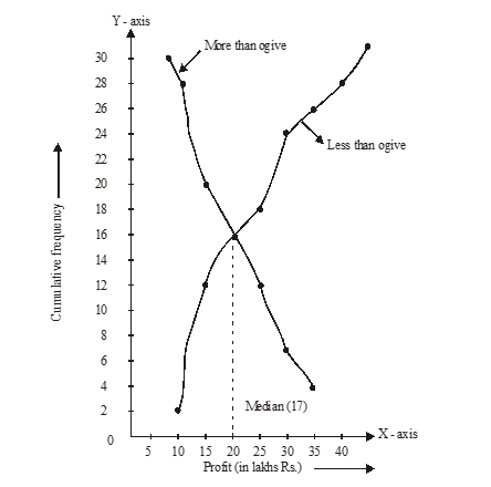
The abscissa of point of intersection is of two curves 17 hence, median = 17