


1. CONCEPT OF LIMITS
1. INTRODUCTION
Consider the function . Clearly f(x) is not defined at x = 1. At x = 1, , which is meaningless.
|
X |
.9 |
.99 |
.999 |
.9999 |
.99999 |
|
f(x) |
1.9 |
1.99 |
1.999 |
1.999 |
1.99999 |
From the above table it is clear that as x approaches to 1 i.e. x 1 from the left hand side (means
x approaches 1 from the values less than 1) f(x) approaches to 2 i.e. f(x) 2. The number 2 is called the left limit of f(x) and in symbol we shall write
Again let us study the behaviour of f(x) where x approaches towards 1 from the right-hand side.
|
X |
1.1 |
1.01 |
1.001 |
1.0001 |
1.00001 |
|
f(x) |
2.1 |
2.01 |
2.001 |
2.0001 |
2.00001 |
It is clear from the table that as x approaches to 2 i.e. x 2, from the right-hand side (means x
approaches 1 from the values greater than 1) f(x) approaches to 2 i.e. f(x) 2. Here 2 is called the
right-hand limit of f(x) and in symbol we will write
Thus we see that f(x) is not defined at x = 1 but its left-hand limit and right-hand limit as x 1 exist and are equal. When are equal we say exist and is equal to 2.
2. MEANING OF ‘ x a ’
Let x be a variable and ‘a’ be a constant. If x assumes values nearer and nearer to ‘a’ but x is strictly
smaller than ‘a’ then this statement is mathematically written as .
Similarly, , implies that x assumes values nearer and nearer to ‘a’ but x is strictly greater
than ‘a’.
In general by ‘x tends to a’ we mean that
(i) x ≠ a
(ii) x assumes values nearer and nearer to ‘a’ and
(iii) we are not specifying the manner in which x should approach to ‘a’.
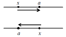
x may approach to ‘a’ from left or right as shown in figure.
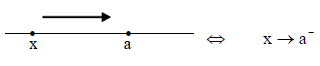
If ‘x’ approach to ‘a’ from any point on the right of x = a in the real number line (i.e. the x axis) but
it never crosses x = a , then it is written as .
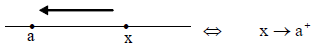
Similarly,
3. NEIGHBOURHOOD OF ‘x = a ’
For some h > 0, sufficiently small, let the function y=f(x) be defined in the interval (a − h, a) then it is said that the function y = f(x) is defined in the left-neighbourhood of x = a.
Similarly, if the function y = f(x) be defined in the interval (a, a + h) then it is said that the function
y = f(x) is defined in the right-neighbourhood of x = a.
If the function y = f(x) be defined in left-neighbourhood of x = a or right-neighbourhood of x = a,
then it is said that the function y = f(x) is defined in the neighbourhood of x = a .
It must be noted here that the value ‘a’ itself may or may not be included in the domain which is
actually not being considered in its neighbourhood.
4. INDETERMINATE FORMS
Some times we come across some functions which do not have definite value corresponding to some particular value of the variable.
For example, the function f(x) = , converts into if x = 2 is substituted.
Hence, f (2) cannot be determined. Such a form is called an Indeterminate Form.
There are total 7 Indeterminate Forms given as
(1) , (2) , (3) , (4) , (5) , (6) , (7)
Note : Here 0 and 1 are all approaching values, not the exact values.
Illustration-1
Which of the following are forming indeterminate form. Also indicate the form
(i)
(ii)
(iii)
(iv)
(v)
(vi)
(vii)
(viii)
Solution
(i) No
(ii) form
(iii) 0 × form
(iv) form
(v) (0)º form
(vi) ()º form
(vii) form
(viii) form
5. LIMIT OF A FUNCTION
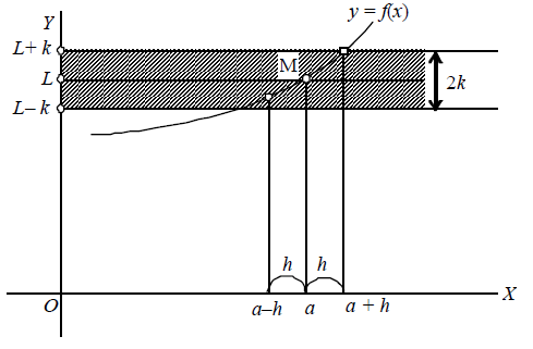
Definition-1
Let the function y = f(x) be defined in a certain neighbourhood of a point x = a . The function y = f(x) approaches the limit L (y L) as x approaches ‘a’ (x a). If for every positive number h, arbitrarily small, we are able to indicate k > 0, arbitrarily small, such that for all x, different from ‘a’ and satisfying the inequality.
we have the inequality
then
or f(x) L as x a or limiting value of f(x) is L as x a.
Definition-2
Let y = f (x) be a function of x and the limiting value of y is required for x a, then we consider the values of the function at the points which are very near to ‘a’.
If these values tend to a definite unique number L as x tends to ‘a’ (either from left or from right)
then this unique number L is called the limit of f(x) at x = a and we write it as
Illustration-2
Evaluate
Solution
x + 2 being a polynomial in x, its limit as x 2 is given by
Illustration-3
Evaluate
Solution
x(x – 1) being a polynomial in x, its limit as x 2 is given by
Illustration-4
Evaluate
Solution
Illustration-5
Evaluate
Solution
Illustration-6
Find the limiting value of .
Solution
At x = 3, converts into an indeterminate form of .
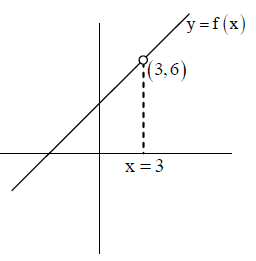
Now when x tends to 3 from left or from right, it can be easily observed from the graph that the value of f(x) tends to 6.
Hence
6. LEFT HAND AND RIGHT HAND LIMIT
Consider the values of the functions at the points which are very near to a on the left of a. If these
values tend to a definite unique number as x tends to a, then the unique number so obtained is called left-hand limit of f(x) at x = a and symbolically we write it as
which is expressed as .
7. EXISTENCE OF LIMIT
The limit of a function f(x) at a point x = a exists and equals to L if finite value, L.
Here are called left hand limit (L.H.L.) and right hand limit (R.H.L.)
respectively.
Thus, if exists then finite value, L L.H.L. = R.H.L. = L
Illustration-7
The value of is, where [ ] represents the greatest integer function.
(A) 1 (B) 2 (C) 4 (D) Does not exist
Solution
Left hand limit =
and Right hand limit =
=
∴ limit does not exist.
Illustration-8
If then at x = 0
(A) right hand limit of f(x) exists but not left-hand limit
(B) left-hand limit of f(x) exists but not right- hand limit
(C) both limits exists but are not equal
(D) both limits exist and are equal
Solution
∴ Both limits exist but are not equal.
Illustration-9
Find
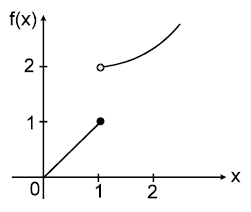
Solution
Left hand limit = 1
Right hand limit = 2
Hence does not exist.
Illustration-10
From the adjoint graph of y = f(x), find
(i)
(ii)
(iii)
(iv)
(v)
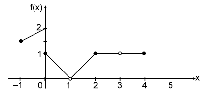
Solution
(i) Here L.H.L. = 2 and R.H.L. = 1
does not exist
because left hand limit ≠ right hand limit.
(ii)
(iii)
(iv)
(v)
8. EVALUATION OF LEFT HAND AND RIGHT HAND LIMITS
Right-hand limit means tendency of function when we approach x = a from the value which just greater than ‘a’ and we write .
Working rule to evaluate
• Put x = a + h in f(x) to get
• Take the limit as h 0
Left-hand limit means tendency of function when we approach x = a from the values which are just less than ‘a’ and we write .
Working rule to evaluate
• Put x = a – h in f(x) to get
• Take the limit as h 0
Illustration-11
If .
Find left and right hand limits and choose whether f (x) has limit at the point x = 0.
Solution
Illustration-12
If f(x) = if x 1
x if 1 < x 2
x–3 if x > 2
Find left and right hand limits and check whether f(x) has limit at the point x = 1 ; 2.
Solution
Now,
does not exists.
3. DIFFERENCE BETWEEN THE VALUE OF A FUNCTION AT A POINT AND THE LIMIT AT A POINT
Case 1: and f(a) both exist but are not equal.
Example
f(x) exists at x = 1
f(1) = 0, value of f also exist at x = 1
But
Case 2: and f(a) both exist and are equal.
Example
f(x) =
, limit exists, and f(1) = (1)2 = 1 Value of also exist.
4. THEOREMS ON LIMITS AND EVALUATION OF ALGEBRAIC LIMITS
1. FUNDAMENTAL THEOREMS ON LIMITS
The following theorems are very useful for evaluation of limits if (l and m are real numbers) then
(1) (Sum rule)
(2) (Difference rule)
(3) (Product rule)
(4) (Constant multiple rule)
(5) (Quotient rule)
(6) If
(7)
(8) If
(9)
(10) If p and q are integers, then , provided is a real number.
(11) If provided ‘f ’ is continuous at , only if l > 0.
2. EVALUATION OF LIMITS INVOLVING ALGEBRAIC FUNCTIONS.
To evaluate the limits involving algebraic functions we use the following methods:
1) Direct substitution method
2) Factorisation method
3) Rationalisation method
4) Application of the standard limit
1. Direct substitution method
This method can be used in the following cases :
i) If f(x) is a polynomial function, then .
ii) If where P(x) and Q(x) are polynomial functions then , provided Q(a) ≠ 0.
Illustration-13
Find
Solution
.
Illustration-14
Find
Solution
.
2. Factiorisation Method
This method is used when turns out to be an indeterminate form of the type by the substitution of x = a.
In such a case the numerator (Nr.) and the denominator (Dr.) are factorised and the common factor (x – a) is cancelled. After eliminating the common factor the substitution x = a gives the limit, if it exists.
Illustration-15
Evaluate .
Solution
=
=
Illustration-16
Evaluate .
Solution
(Cancelling the common factor (x–2)).
3. Rationalisation Method
This method is used when is a form and either the Nr. or Dr. consists of expressions
involving radical signs.
Illustration-17
Show that
Solution
= = .
Illustration-18
Evaluate
Solution
=
=
=
= .
4) Application of the standard limit
This method is explained through the following examples.
Illustration-19
Compute
Solution
= .
Illustration-20
Find
Solution
Let 2 + x = t. Then .
.
Illustration-21
Show that .
Solution
=
Put a + x = t in (i) and a – x = s in (ii) then x 0 t a, s a
∴ Given limit =
= .
Note:
i) .
ii) .
iii) .
Illustration-22
Evaluate .
Solution
=
= .
5. EVALUATION OF TRIGONOMETRIC LIMITS
To evaluate trigonometric limit the following results are very important.
(i)
(ii)
(iii)
(iv)
(v)
(vi)
(vii)
(viii)
(ix)
(x)
(xi)
(xii)
(xiii)
Illustration-23
Find
Solution
=
Note:
.
Illustration-24
Find
Solution
= = 1.a – 1. b = a – b.
Illustration-25
Evaluate
(i)
(ii)
Solution
(i) radians radians
=
(ii) .
(Where t = and x 0 t 0)
Illustration-26
Find
Solution
Let x – a = t then x a t 0; x + a = t + 2a
= .
Illustration-27
Evaluate
Solution
Illustration-28
Evaluate
Solution
Illustration-29
Evaluate
Solution
.
= = .
Illustration-30
Compute
Solution
=
= .
Illustration-31
Find
Solution
Put then
= .
Illustration-32
Show that
Solution
= = a (where t = ax)
Illustration-33
Show that
Solution
Let so that x = sint, then x 0 t 0
.
Illustration-34
Show that
Solution
= .
Illustration-35
Show that does not exist.
Solution
As x 0, LHL ≠ RHL
does not exist.
6. EVALUATION OF EXPONENTIAL AND LOGARITHMIC LIMITS
1. LOGARITHMIC LIMITS
To evaluate the logarithmic limits we use following formulae
(i) where and expansion is true only if base is e.
(ii)
(iii)
(iv)
(v)
2. EXPONENTIAL LIMITS
i. Based on series expansion
We use
To evaluate the exponential limits we use the following results
(a)
(b)
(c)
ii. Based on the form :
To evaluate the exponential form we use the following results.
(a) If , then
or when and .
Then =
(b)
(c)
(d)
(e)
• , if a > 1 and if a < 1.
Illustration-36
Evaluate .
Solution
=
= = log 9. log3
Illustration-37
Evaluate .
Solution
= = .
Illustration-38
Evaluate where a, b are constants.
Solution
We know that .
Now,
, (where t = ax)
=
Aliter:
The given limit is of the form .
Illustration-39
Evaluate where a,b,c,d are positive constants.
Solution
( form)
= =
Aliter: =
=
Illustration-40
Find
Solution
The given limit is of form
= = .
Illustration-41
Find , a, b are constants.
Solution
=
=
= , where
= .
Illustration-42
Evaluate where a,b,c,d are constants.
Solution
=
=
Illustration-43
Evaluate where a,b,c
Solution
The given limit is of
=
=
= .
Note :
i) .
ii) .
Illustration-44
If , find a and b.
Solution
=
= = , for any
7. EVALUATION OF LIMITS BY USING DE’L’ HOSPITAL’S RULE
1) Let f(x) and g(x) be two functions such that
Then provided the latter limit exists. (Here ‘ denotes differentiation wrt x)
2) Let f(x) and g(x) be two functions such that .
Then provided the latter limit exists.
Note:
i) L’ Hospital’s rule can be applied repeatedly i.e., provided these limits exist and at each stage of application of the rule, we should make sure that the limit is either a from or an form.
ii) While applying the L’Hospital’ s rule the derivatives of the Numerator f(x) and the Denominator g(x) w.r.t x are to be calculated separately and at the same time, but not by using quotient rule on f(x) / g(x).
iii) L’Hospital’s rule is directly applicable to and forms only. This rule is not applicable directly to other indeterminate forms. but can be applied only after transforming them into either form or form.
Illustration-45
Find
Solution
.
Illustration-46
Evaluate .
Solution
.
Illustration-47
Find .
Solution
.
Illustration-48
If is finite find the values of a and b. Also find the limit.
Solution
Let
This can be finite only if 1 + a + b = 0 — (1)
(applying L’ Hospital’s rule)
(applying L’ Hospital’s rule) =
This can be finite only if – 16 – 4a = 0 — (2)
From (2), a = – 4
From (1), b = 3 a = –4, b = 3.
Now, required limit is
=
.
8. SOME USEFUL RESULTS AND FREQUENTLY USED EXPANSIONS
1. SOME USEFUL RESULTS
i. Let S = {x,sin x, tan x,sinh x, tanh x,sin-1 x, tan-1 x,sinh-1 x, tanh-1 x}
If f (x), g(x)S then
If then
ii.
2. EVALUATION OF LIMITS USING SERIES EXPANSIONS
In the evaluation of certain limits it becomes necessary to use the following series expansions:
i)
ii) +….(a>0, xR)
iii)
iv)
v)
vi)
vii)
viii)
ix)
x)
xi)
xii)
xiii)
Illustration-49
Find .
Solution
(terms containing positive integral powers of x)
.
Illustration-50
Find the values of a,b and c if
Solution
The limit is finite and is equal to 2 only if
a – b + c = 0 — (1), a – c = 0 — (2)
and …..(3)
Solving (1) (2) and (3), a = 1, b = 2, c = 1.
Illustration-51
Evaluate
Solution
=
= =
= (+term containing positive powers of x)
= .
9. SANDWICH THEOREM OR SQUEEZE PRINCIPLE
If & then
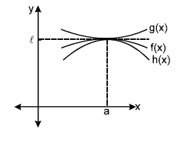
Illustration-52
Evaluate , Where [ ] denotes the greatest integer function.
Solution
We know that, x – 1 < |x| x
(x + 2x + 3x + …. + nx) – n < [x] + [2x] + ….. +[nx] (x + 2x + …. + nx)
Thus,
<
Illustration-53
Find .where [.] denotes the GIF.
Solution
For any x R, we know that x – 1 < [x] x
.
10. MISCELLANEOUS CONCEPTS AND PROBLEMS
1. METHOD OF EVALUATING LIMITS OF ALGEBRAIC FUNCTIONS OF X WHEN
We make use of the following basic limits.
i) (k is a constant)
ii) If n>0 then
iii) If , then ,
Illustration-54
Evaluate
Solution
Illustration-55
Find
Solution
2. EVALUATION OF INFINITE LIMITS
In evaluating this type of limits, we use the following basic results on limits :
i) = does not exist.
ii) ,
does not exist. For a positive integer, n
iii)
iv) , .
v) , .
vi) .
vii) .
viii) If and f(x) > 0 in a deleted nbd of a then .
ix) If and f(x) < 0 in a deleted nbd of a then .
x) If then may or may not exist.
Illustration-56
Find
Solution
Since and
the given limit can not be finite.
For x ≠ 3, and in a nbd, of the point 3.
Let . Then f(x)>0 in a deleted nbd of 3 and
Hence .
3. EVALUATION OF LIMITS OF FORM :
i) If is of the form , it can be transformed to or form by writing it as and hence can be evaluated.
iii) If is of the form or , it can be expressed as so that the limit in the exponent is a 0. and hence can be evaluated as in (ii).
Illustration-57
Determine
Solution
.
Illustration-58
Find
Solution
=
=
= .
Illustration-59
Evaluate .
Solution
, say
Then
=
.
Illustration-60
Solution
Let
Then log y = tan x log
Then,
=
.
11. DERIVATIVES
We know that the tangent line to the curve y = f(x) at the point (a,f(a)) has slope

The derivative of the function f is the function f ‘ define by for all x for which this limit exist.
Illustration-61
Find the derivative of .
Solution
We have =
12. DERIVATIVES OF SOME OF THE FREQUENTLY USED FUNCTIONS
|
Function |
Derivative |
|
c (constant) |
0 |
|
sinx |
cosx |
|
cos x |
–sinx |
|
tanx |
sec2x |
|
xn |
nxn–1 |
The above written derivatives can be easily found by using the definition of differentiation.
13. RULES TO FIND OUT DERIVATIVES
Let u and v are differentiable functions of ‘x’.
(i) The sum rule
e.g.
(ii) Product rule
e.g.
= (sinx) ex + (cosx) ex.
Illustration-62:
Differentiate .
Solution:
First we differentiate
Now,
(iii) The quotient rule
Here v(x) ≠ 0
e.g.
Illustration-63:
Differentiate
Solution:
(iv) Chain rule
The chain rule is probably the most widely used differentiation rule in mathematics. Chain rule says that the derivative of the composite of two differentiable functions is the product of their derivatives evaluated at appropriate points.
The formula is
Illustration-64:
Differentiate
Solution:
Put and z = siny
Then
=
This solution can be rewritten using a more convenient notation in the following manner:
=
Illustration-65:
Differentiate with respect to x.
Solution:
Let