Units and Measurements

1. PHYSICAL WORLD

Physics deals with the study of the basic laws of nature and their manifestation in different phenomena. The basic laws of physics are universal and are applied in widely different contexts and conditions.

Physics, Technology and Society

• Science, Technology and Society have strong relationships among one on other. Science is the mother of technology and both of them are the reasons for the creation and development of the society.
• Science and technology issues are actually discussed worldwide today. Progress in this has led to produce the ability to integrate different types of physical products.
• Physics is a basic discipline in the category of natural sciences which also includes other disciplines like Chemistry and Biology. The word physics comes from a Greek word meaning nature.
• Some physicists from different countries of the world and their major contributions

LIST OF IMPORTANT NOBEL PRIZES
Name of Scientist	Year of Award	Contribution for which Nobel Prize is awarded
Wilhelm Konrad Roentgen	1901	the discovery of X-rays.
AH. Becquerel	1903	the discovery of spontaneous radioactivity.
G.Marconi	1909	the contribution to the development of wireless.
H.K Onnes	1913	the investigations of the properties of matter at low temperatures.
Max Planck	1918	the discovery of energy quanta
Albert Einstein	1921	his services to Theoretical Physics, and especially for his discovery of the law of photoelectric effect.
N.Bohr	1922	the investigation of the structure of atoms, and of the radiation emanating from them.
R.A. Millikan	1923	his work on the elementary charge of electricity and on the photoelectric effect.
A.H. Compton	1927	his discovery of the effect named after him.
Louis-Victor de Broglie	1929	the discovery of the wave nature of electrons.
Sir Chandrasekhara Venkata Raman	1930	his work on the scattering of light and for the discovery of effect named after him.
Werner Heisenberg	1932	the creation of quantum mechanics.
James Chadwick	1935	the discovery of neutron
Victor Franz Hess	1936	the discovery of cosmic radiation
Enrico Fermi	1938	the demonstration of the existence of new radioactive elements.
Wolfgang Pauli	1945	the discovery of Exclusion principle (Pauli principle)
Hideki Yukawa	1949	the prediction of the existence of mesons on the basis of theoretical work on nuclear forces.
William Shockley, John Bardeen, W.H. Brattain	1956	their researches on semi-conductors and their discovery of the transistor effect.
H.A. Bethe	1967	his contribution to the theory of nuclear reac­tion, especially his discoveries concerning the energy production in stars.
Dennis Gabor	1971	the discovery of the principle of holography.
J. Bardeen, L.N. Cooper, J.R. Schrieffer	1972	the development of a theory of supercon­ductivity.
S.L. Glashow, Abdus Salam, S. Weinberg	1979	their unified model of the action of the weak and electromagnetic forces and for their prediction of the existence of neutral currents.
Ernst Ruska	1986	his invention of the electron microscope.
Karl Alex Miiller, J.G. Bednorz	1987	their discovery of a new class of super­conductors
Pierre-Gilles de Gennes	1991	discoveries about the ordering of molecules in substances such as liquid crystals, supercon­ductors and polymers.

 

List of Important Discoveries
Name of Discoverer	Nationality	Contribution/Discovery	Year
Copernicus	Poland	Sun as centre of solar-system	1543
Galileo	Italy	Law of Falling bodies	1590
Hans Lippershey	Netherlands	Telescope	1608
Johannes Kepler	Germany	Laws of Planetary Motion	1609-1619
John Napier	Scotland	Logarithms	1614
E. Torricelli	Italy	Barometer	1643
Dennis Papin	France	Pressure Cooker	1675
Issac Newton	England	Laws of gravitation and Motion	1687
Thomas Newcomen	England	Steam Engine	1712
G. Fahrenheit	Germany	Mercury thermometer	1714
Benjamin Franklin	USA	Lightning conductor	1752
James Watt	Scotland	Condensing Steam Engine	1765
C.A. Vatta	Italy	Electric Battery	1800
K.V. Sauerbronn	Germany	Bicycle	1816
William Sturgeon	England	Electromagnet	1825
Michael Faraday	England	Dynamo and Law of Electromagnetic Induction	1831
Elisha Otis	USA	Passenger lift	1853
F. Caree	France	Refrigerator	1858
E. Lenoir	France	Internal combustion Engine	1859
Graham Bell	Scotland	Telephone	1876
David Edward Hughes	England/USA	Microphone	1878
James Dewar	Scotland	Vacuum Flask	1885
William Stanley	USA	Electric Transformer	1885
H. Hertz	Germany	Electromagnetic waves	1886
G.Marconi	Italy	Wireless	1895
W. Roentgen	Germany	X-rays	1895
Antoine Becquerel	France	Radioactivity	1896
Rudolf Diesel	Germany	Diesel Engine	1897
Pierre and Marie Curie	France	Radium	1898
Max Planck	Germany	Quantum theory	1900
Wilbur Orville Wright	USA	Aeroplane	1903
John Fleming	England	Diode	1904
Lee De Forest	USA	Triode	1906
Albert Einstein	Switzerland	General theory of Relativity	1915
H.C. Oersted	Denmark	Electro-magnetism	1920
John Baird	Scotland	Television	1925
Robert H. Goddard	USA	Rocket (Liquid Fuel)	1926
James Chadwick	England	Neutron	1932
J. Presper Eckert and John W. Mauchly	USA	Electronic Computer	1946
John Bardeen, W. Brattain, W. Shockley	USA	Transistor	1948
Theodore Maiman	USA	Laser	1960

  

Link between Technology and Physics
SN	Technology	Scientific Principles
1	Aeroplane	Bernoulli’s principle in fluid dynamics
2	Bose-Einstein condensate	Trapping and cooling of atoms by laser beams and magnetic fields
3	Computers	Digital logic
4	Steam engine	Laws of thermodynamics
5	Nuclear reactor	Controlled nuclear fission
6	Radio and Television	Generation, propagation and detection of electromagnetic waves
7	Lasers	Light amplification by stimulated emission of radiation
8	Production of ultra-high magnetic fields	Superconductivity
9	Rocket propulsion	Newton’s laws of motion
10	Electric generator	Faraday’s laws of electromagnetic induction
11	Hydroelectric power	Conversion of gravitational potential energy into electrical energy
12	Particle accelerators	Motion of charged particles in electromagnetic fields
13	SONAR	Reflection of ultrasonic waves
14	Optical fibres	Total internal reflection of light
15	Non-reflecting coatings	Thin film optical interference
16	Electron microscope	Wave nature of electrons
17	Photocell	Photoelectric effect
18	Fusion test reactor (Tokamak)	Magnetic confinement of plasma
19	Giant Metrewave RadioTelescope ( GMRT)	Detection of cosmic radio waves
20

 Fundamental forces in nature

• There are four fundamental forces in nature. They are the ‘gravitational force’, the ‘electromagnetic force’, the ‘strong nuclear force’, and the ‘weak nuclear force’. Unification of different forces/domains in nature is a basic quest in physics.

Nature of physical laws

• The physical quantities that remain unchanged in a process are called conserved quantities. Some of the general conservation laws in nature include the laws of conservation of mass, energy, linear momentum, angular momentum, charge, Some conservation laws are true for one fundamental force but not  for the  other.
• Conservation laws have a deep connection with symmetries of nature. Symmetries of space and time, and other types of symmetries play a central role in modern theories of fundamental forces in nature.

2. MEASUREMENT AND UNITS:

Physics is a basic discipline in the category of Natural Sciences, which also includes other disciplines like Chemistry and Biology.  The word Physics comes from a Greek word ‘FUSIS’ meaning nature.  Physics is the study of nature and its laws.  We expect that all these different events in nature take place according to some basic laws and revealing these laws of nature from the observed events in Physics.

Physics is quantitative science.  To describe any physical phenomenon, measurements of different physical quantities is essential.  Measurement of any physical quantity involves comparison with certain basic, arbitrary chosen, internationally accepted reference standard called unit.

Measurement of any physical quantity involves comparison with certain basic, arbitrary chosen, internationally accepted reference standard called unit.

To measure a physical quantity we need some standard unit of that quantity.  The measurement of the quantity is mentioned in two parts, the first part gives how many times of the standard unit and second part gives the name of the unit.  Thus, suppose I say that length of this wire is 5 metres.  The numeric part 5 says that it is 5 times of the unit of length and the second part ‘metre’ says that the unit chosen here is metre.

3. FUNDAMENTAL AND DERIVED PHYSICAL QUANTITIES

There are a large number of physical quantities which are measured and every quantity needs a definition of unit.  But, not all the quantities are independent of each other.  Therefore, the physical quantities which can exist independently are called fundamental quantities.  For example length, mass etc.  All other quantities may be expressed in terms of fundamental quantities are called derived physical quantities.  For example force, density etc.

4. SI SYSTEM OF UNITS

It is abbreviated as S.I. from the French name Le system International d’ unites.  Table below gives the seven fundamental quantities and their S.I. Units.

S. no.	Quantity	S.I. Unit	Symbol
1	Length	metre	m
2	Mass	kilogram	kg
3	Time	second	s
4	Electric Current	ampere	A
5	Temperature	kelvin	K
6	Amount of substance	mole	mol
7	Luminous Intensity	candela	Cd

Two supplementary quantities namely, plane angle and solid angle are also defined.  Their units are radian (rad) and steradian (sr) respectively.

Definition of Units in S.I.

i) metre(m): This is the unit of length. The value of metre is taken as the distance travelled by light in vacuum during a time interval of 1/299 792 458^th of a second.

ii) kilogram (kg): This is a unit of mass. It is the mass of a cylinder (prototype) made of Platinum iridium alloy kept at International Bureau of Weights and Measures.

iii) second (s): This is unit of time. It is defined as the duration of 9,192,631,770 periods of the radiation corresponding to the transition between the two hyperfine levels of the ground state of the Caesium-133 atom.

iv) ampere (A): This is unit of electric current. Consider two infinitely long parallel straight conductors of negligible circular cross- section separated by one metre distance in vacuum.  Then, the magnitude of electric current passed in each of these conductors to produce a force of 2×10^-7 N/m between them is called an ampere.

v) kelvin(K): This is the unit of temperature. The fraction $\frac{1}{273.16}$ of the thermodynamic temperature of triple point of water.

vi) candela (Cd): It is the luminous intensity of a black body of surface area $\frac{1}{600,000}$ m² placed at the temperature of freezing platinum and at a pressure of 101,325 N/m² in the direction perpendicular to its surface.  It is the unit of luminous intensity.

vii) mole(Mol): It is defined as the amount of a substance which contains as many elementary entities as there are atoms in 12 g of carbon-12 (C¹²).  It is the unit of quantity of substance.

viii) radian(rad): It is defined as the angle subtended at the centre of a circle by an arc whose length is equal to the radius of the circle is known as radian.  It is the unit of plane angle. $\mathrm{\pi }$ radian = 180^o or 1 radian = $\frac{180}{\pi }=57°{19}^1{45}^{11}$

ix) steradian (sr): Steradian is defined as the solid angle subtended at the centre of the sphere by its surface whose area is equal to the square of the radius of the sphere. If dA is area intercepted by solid angle , then  where R is the radius of curvature of spherical surface.

5. MULTIPLES AND SUBMULTIPLES OF SI UNITS

The magnitude of physical quantities vary over a wide range.  We talk of separation between two protons inside a nucleus which is about 10^-15 m and distance of a quasar from the earth which is about 10²⁶ m.  To measure very low or very high values of physical quantities prefixes are used to represent them.  For example 10^-3 m is written as 1 millimeter.

Multiplication factor	Prefix	Symbol	M.F.	Prefix	Symbol
10-1	deci	d	101	deka	da
10-2	centi	c	102	hecta	H
10-3	milli	m	103	kilo	K
10-6	micro	$\mu$	106	mega	M
10-9	nano	n	109	giga	G
10-12	pico	p	1012	tera	T
10-15	femto	f	1015	peta	P
10-18	atto	a	1018	exa	E
10-21	zepto	z	1021	zetta	Z
10-24	Yacto	y	1024	yotta	Y

6. DIMENSIONAL ANALYSIS

The dimensions of a physical quantity is the powers to which the fundamental units of mass, length and time have to be raised to represent a derived unit of the quantity.

The dimensional formula of a physical quantity is an expression which tells us:

i) The fundamental quantities on which the quantity depends, and

ii) The nature of the dependence For example [M^oL¹T^-1] is the dimensional formula of velocity.  It reveals that unit of velocity depends on [L] and [T].  It does not depend on [M].  Further, unit of velocity varies directly with unit of length and inversely as unit of time. From the study of dimensional formulae of various quantities, we can easily divide them into four types.

1. Dimensional constants: These are the quantities whose values are constant and they possess dimensions.  For example, velocity of light in vacuum, universal gravitational constant, Planck’s constant etc.

2. Dimensional Variables: These are the quantities whose values are variables, and they possess dimensions. For example, area, volume, force etc. dimensions.  For example 1, 2……. $\mathrm{\pi }$ , e etc.

3. Dimensionless variables: These are the quantities whose values are variables and they do not possess dimensions.  For example angle, strain etc.

S. No.	Physical Quantity	Expression	Dimensional formula	Units
1	Density (D)	Mass/Volume	[ML–3T0]	kgm–3
2	Relative density (specific gravity)	Density of substance/Density of water	[M0L0T0] Dimensionless	–
3	Frequency(f)	Vibrations/time	[M0L0T-1]	Hz
4	Angle	Arc/radius	[M0L0T0] Dimensionless	–
5	Velocity (v)	Displacement/time	[M0L1T-1]	ms-1
6	Angular velocity ( $\omega$)	Angle/time	[M0L0T-1]	rad s-1
7	Acceleration (a)	Change in velocity/time ( $∆$v/ $∆$t)	[M0L1T-2]	ms–2
8	Angular acceleration	$∆\omega$/ $∆$t	[M0L0T-2]	rad s–2
9	Linear momentum	Mass x velocity	[M1L1T-1]	kgms-1
10	Angular momentum	Momentum x arm	[ML2 T-1]	Kgm2s–1
11	Force(F)	Mass x acceleration	[MLT-2]	N
12	Torque	Force x arm	[ML2T-2]	kg m2s–2 or Nm
13	Impulse	Force x time	[MLT-1]	Ns or Kg ms-1
14	Pressure	Force/area	[ML–1T-2]	Nm–2 or Pa
15	Work, Potential energy, Kinetic energy	$\frac{1}{2}m{v}^2$Force x distance	[ML2 T-2]	Nm or J
16	Gravitational constant (G)	$\frac{\text{ force }\times (\text{ Length }{)}^2}{(mass{)}^2}$	[M-1L3T-2]	Kg-1 m3 s–2
17	Planck’s constant (h)	Energy/Frequency	[M1L2 T-1]	Kg m2s-1 or Js
18	Power	Work/Time	[ML2T–3]	W or Js–1
19	Moment of Inertia	Mass x (distance)2	[ML2T0]	Kgm2
20	Stress	Force/Area	[ML–1T–2]	Nm–2 or Pa
21	Strain	Change in Length/Original length	[M0L0T0] dimensionless
22	Modulus of Elasticity	Stress/Strain	[ML–1T–2]	Nm–2
23	Velocity gradient	Change of velocity/distance	[M0L0T–1]	s-1
24	Coefficient of Viscosity	Tangential Stress/Velocity gradient	[ML–1T–1]	Kgm-1s-1 or Nm-2s or Pas
25	Surface Tension	Force/Length	[ML0T–2]	Kg s–2 or Nm–1
26	Specific heat	$\frac{\text{ Enegry }}{\text{ Mass }\times \text{Temp }}$	[M0L2T–2K–1]	J Kg-1 K-1
27	Latent Heat	Energy/Mass	[M0L2T–2]	J Kg-1
28	Universal gas constant (R)	$\frac{\text{ Energy }}{\text{ Temp-Mol }}$	[ML2T–2 K-1mol-1]	JK-1 mol-1
29	Boltzmann’s constant	Energy/Temp	[ML2T–2K-1]	JK-1

7. APPLICATIONS OF DIMENSIONAL ANALYSIS Dimensional formulae are used:

i) to convert one system of units into another

ii) to check the correctness of an equation

iii) to derive relationship between different physical quantities.

Let us discuss in a little more detail, the uses of dimensional formulae mentioned above.

i) Conversion of one system of units to another:

Let the dimensional formula of physical quantities is [M^aL^bT^c].  Let n₁ be its numerical value in one system in which units of fundamental quantities are M₁, L₁ and T₁.  Then the numerical value n₂ in another system in which units of fundamental quantities are M₂, L₂ and T₂, is given by

n₂[M₂^aL₂^bT₂^c] = n₁[M₁^aL₁^bT₁^c]

or, ${\mathrm{n}}_2={\mathrm{n}}_1{\left(\frac{{\mathrm{M}}_1}{{\mathrm{M}}_2}\right)}^a{\left(\frac{{\mathrm{L}}_1}{{ \mathrm{L}}_2}\right)}^{\mathrm{b}}{\left(\frac{{\mathrm{T}}_1}{{ \mathrm{T}}_2}\right)}^{\mathrm{c}}$

Therefore, as the fundamental units in both the systems are known, we can determine numerical value in one system if the numerical value in the other system is known. Let us find the relation between units of force.  Newton is unit of force in S.I. and dyne is its unit in C.G.S. system.

Dimensional formula of force is [M¹L¹T^-2].

Let 1N = n dynes    or, n = 1 N/dynes

Hence $\mathrm{n}=\left(\frac{{\mathrm{M}}_1}{{\mathrm{M}}_2}\right)\left(\frac{{\mathrm{L}}_1}{{ \mathrm{L}}_2}\right){\left(\frac{{\mathrm{T}}_1}{{ \mathrm{T}}_2}\right)}^{–2}$

In S.I. unit: M, L and T are kg, m and s and in C.G.S. unit: M, L and T are gm, cm and s.

$\therefore \mathrm{n}=\left[\frac{\mathrm{kg}}{1\mathrm{gm}}\right]\left[\frac{1 \mathrm{m}}{1 \mathrm{cm}}\right]{\left[\frac{1 \mathrm{s}}{1 \mathrm{s}}\right]}^{–2}$ = $\left[\frac{1000\mathrm{gm}}{1\mathrm{gm}}\right]\left[\frac{100 \mathrm{cm}}{1 \mathrm{cm}}\right]{\left[\frac{1 \mathrm{s}}{1 \mathrm{s}}\right]}^{–2}$ = (1000) (100) (1) =  10⁵

Hence, 1N = 10⁵ Dynes.

ii) To check the correctness of an equation:

The correctness of equation is verified using the principle of homogeneity of an equation.  The principle states that, terms on both sides of a dimensional equation should have same dimensions.

Let us consider the equation $\mathrm{T}=2\pi \sqrt{\frac{1}{ \mathrm{g}}}$ and check whether it is correct or not. We know that, dimensional formula of t, l and g are [T], [L], [LT^-2] respectively.

$\therefore$ Dimensional formula of $\sqrt{\frac{\mathrm{l}}{\mathrm{g}}}=\sqrt{\frac{\mathrm{L}}{{\mathrm{LT}}^{–2}}}=\sqrt{{\mathrm{T}}^2}=\left[\mathrm{T}\right]$

Dimensional formula of left hand side is also [T].  As 2 $\mathrm{\pi }$ is dimensionless quantity, the dimensional formula of left hand side of the equation is equal to dimensional formula of right hand side.

Hence we conclude that the given equation is a correct one.  In the above equation the value of 2 $\mathrm{\pi }$ cannot be determined from the dimensional analysis but it is to be determined only from the experimental data.

iii) To derive the relationship between different physical quantities:

Let us derive an expression for the velocity of sound in solids.  Let v be the velocity of sound in a solid.  Assuming that it depends upon the density (d) and coefficient of elasticity (E) of the medium,

let v $\propto$ E^a  and v $\propto$ d^b

or, v = k E^ad^b where k is proportionality constant.

Dimensional formula of v, E and d are

v = [M^o L T^-1]

E = [ML^-1 T^-2]

d  = [ML^-3T⁰]

Using dimensional analysis

[M⁰LT^—1] = [ML^—1T^—2]^a[ML^-3T⁰]^b where k has no dimensions.

or, [M⁰LT^-1] = [M^a+bL^-a-3bT^-2a]

We get a+b = 0

-3b-a = 1

and   -2a = -1 or a = 1/2

then, a = 1/2, b = – ½

8. PRINCIPLE OF HOMOGENEITY OF DIMENSIONS

If x = y+z is dimensionally correct and if x represents the physical quantity, the force, then y and z also must represent the same physical quantity i.e. force.  It means the terms of both sides of a dimensional equation should have same dimensions.  This is called principle of homogeneity of dimensions.

9. LIMITATIONS OF DIMENSIONAL ANALYSIS

Dimensional methods are very simple and convenient for arriving at equations connecting physical quantities.  But they have certain limitations.

i) The value of dimensionless constants or proportionality constants cannot be found by dimensional methods. They have to be determined experimentally.

ii) The equation containing trignometrical, exponential and logarithmic function cannot be analysed.

iii) If the physical quantity is sum or difference of two or more quantities, we cannot use dimensional methods.  It is just possible to verify the relation dimensionally.

iv) In some cases proportionality constants have dimensions. Then we cannot apply dimensional methods to derive the formulae.

For example $\mathrm{F}=\mathrm{G}\frac{{\mathrm{m}}_1{ \mathrm{m}}_2}{{\mathrm{r}}^2}$ cannot be derived by dimensional methods.

v) It is difficult to apply dimensional methods if the physical quantity depends upon more than three fundamental quantities length, mass and time.

ERROR ANALYSIS

10. SIGNIFICANT FIGURE

Significant figures in the measured value of a physical quantity tell the number of digits in which we have confidence.  Larger the number of significant figures obtained in a measurement, greater in the accuracy of the measurement or vice versa.

Common rules for counting significant figures

Following are the common rules in a given expression.

Rule 1: All the non-zero digits are significant.

Rule 2: All the zeros occurring between two non-zero digits are significant, no matter where the decimal point is, if at all.

Rule 3: In a number less than one, all the zeros to the right of decimal point and to the left of the point non-zero digit are not significant.

Rule 4: The terminal or trailing zeros in a number without a decimal point are not significant.

Rule 5: The trailing zeros in a number with a decimal point are significant.

Note:

(i): For a number greater than 1, without any decimal, the trailing zeros are not significant.

(ii): For a number with a decimal, the trailing zeros are significant.

11. COMMON RULE FOR ROUNDING OFF

We use the following rules by convention:

Rule 1: If the digit to be dropped is less than 5, then the preceding digit is left unchanged.

Rule 2: If the digit to be dropped is more than 5, then the preceding digit is raised by one.

Rule 3: If the digit to be dropped is 5 followed by digits other than zero, then the preceding digit is raised by one.

Rule 4: If the digit to be dropped is 5 or 5 followed by zeros then the preceding digit is left unchanged, if it is even.

Rule 5: If the digit to be dropped is 5 or 5 followed by zero, then the preceding digit is raised by one, if it is odd.

Note:

i) In multiplication or division, the final result should retain only that many significant figures as are there in the original number with the least number of significant figures.

ii) In addition or subtraction the final result should retain only that many decimal places as are there in the number with the least decimal places.

12. TYPES OF ERRORS

Due to the presence of errors, any measurement made with measuring instruments like a scale, balance or clock will give only approximate values.  Broadly the errors are classified as systematic errors and random errors.  Let us consider some of the errors we usually encounter within our measurements.

Constant Errors:

When the result of a series of  measurements are in error by the same amount, such an error is called constant error.  The constant error arises due to (a) imperfect design (b) zero error in the instrument or any other such defects.  These are also called ‘instrumental errors’.  These errors will be there irrespective of high precision of the instrument.  If a scale is worn off at the starting end up to 0.2 cm reading and we do not notice it and treat it and treat it as zero, then every length we measure will be always 0.2 cm more than the true value.  Same is the case with a faultily calibrated thermometer.  If a screw gauge has a zero error of -4 head scale divisions, then every reading will be 0.004cm less than the true values.

These errors are called constant errors because, with the given instrument the error will be of the same magnitude and same sign (either always positive or always negative).  These constant errors can be determined before hand and the measurements can be corrected for.

Systematic Errors:

Systematic errors are those errors that tend to be always in one direction.  These errors will be always either positive or always be negative.  Systematic errors with a constant magnitude are called constant errors.  Other types of systematic errors are

Imperfection in Experimental Technique or Procedure:

Even when the cause of error is quite well known, sometimes the error cannot be eliminated due to imperfection in experimental arrangement, procedure followed and experimental technique employed.  For example, in calorimetric experiments, the loss of heat due to radiation, the effect on weighing due to buoyancy of air cannot be avoided.  A thermometer placed under the armpit will always show a temperature lower than actual value of the body temperature. These errors will be always present and can be suitably correct for.

Environmental Errors (Errors due to External Causes):

These errors arise due to external conditions, that is, due to changes in the environment.  During the experimental measurement there may be changes in external conditions – changes in temperature, pressure, humidity, wind velocity etc.  These errors systematically affect the measurements.  For example, due to raise in temperature a scale gets expanded and this results in measuring length shorter than the real value.

These errors can be taken care of by applying suitable corrections.

Personal Errors or Observational Errors:

These errors are entirely due to the personal peculiarities of the experimenter.  Individual bias, lack of proper setting of the apparatus, carelessness in taking observations (without taking the required necessary precautions.) etc. are the causes for this type of error.  A person may be habituated to hold his eyes (head) always a bit too far to the right (or left) while taking the readings with a scale.  We know that this will give rise to parallax error.  The more experienced and the more cautious and attentive the observer becomes, the less will be the personal errors.  The effect of these observational errors can be minimized by obtaining several readings with due care and then taking the arithmetic mean of the readings.  The systematic errors can be minimized by

i) selecting better instruments with higher resolution.

ii) taking care to avoid personal bias as far as possible.

iii) Improving the experimental techniques.

Random Errors:

Unlike systematic errors these errors are at random with respect to the sign and magnitude.  The occur irregularly – sometimes increasing, sometimes decreasing with changing magnitudes.  These errors arise due to the random fluctuations in experimental conditions that cannot be predicted.  For example, the random fluctuations in temperature, voltage supply and mechanical vibrations of experimental set up etc. are the causes for random errors.  The diameter of a wire may be varying from position to position along its length due to non uniform cross section.  Hence we get random errors in the measurement of diameter.  At some places the value will be more, at some places less with different magnitudes.  The uneven tightening of the screw in a screw gauge at different places of a wire of uniform cross section also results in random errors. 

Thus, even when the same person repeats the same observation, he may get different readings each time. If we repeat the observations over a large number of times and find the arithmetic mean of all the readings, we get the most accurate or very close to the most accurate reading for that observation. Almost all experimental measurements are subject to both systematic and random errors.

Gross Errors:

While noting down the length of an object, the experimenter may read a value of 4.21 cm but may record it as 2.41 cm or 1.24cm.  This is improper recording.  This results in a gross error.  Other causes for gross errors are (a) neglect of the sources of error and (b) reading the instrument incorrectly.  In a tangent galvanometer experiment, the coil is to be placed exactly in the magnetic meridian and care should be taken to see that no other magnetic materials are present in the vicinity.  Any neglect in taking the precautions results in gross errors.

These grosses errors are the result of sheer carelessness on the part of the observer.  No corrections can be applied to these gross errors.  Care should be taken to avoid such errors.  Taking all precautions that are required, we can minimize gross errors.  Actually these gross errors are to be called mistakes and are to be avoided.

Errors, Accuracy and Precision:

The random errors can be treated by statistical methods.  There are well defined procedures for reducing random errors.  Random errors can be reduced with more care in taking measurements.

When the random errors could be eliminated we say the measurements are ‘precise’.  When all types of errors-systematic, random and gross errors are eliminated we say the measurements are ‘accurate’.  The accurate measurements will be nearer to the true value of the quantity.

Absolute Error

In the measurement of a physical quantity it is the magnitude of the difference between the true value and the measured value of the quantity.  Arithmetic mean of the measured values a₁, a₂, a₃…………a_n is $a_m=\frac{1}{n}\sum _{i=1}^{i=n}{a}_i$

By definition absolute errors are $\Delta {\mathrm{a}}_1={\mathrm{a}}_{\mathrm{m}}–{\mathrm{a}}_1,\Delta {\mathrm{a}}_2={\mathrm{a}}_{\mathrm{m}}–{\mathrm{a}}_2\dots \dots \dots \dots \Delta {\mathrm{a}}_{\mathrm{n}}={\mathrm{a}}_{\mathrm{m}}–{\mathrm{a}}_{\mathrm{n}}$ .  The absolute errors may be positive in certain cases and negative in certain other cases.

Mean absolute Error:

It is the arithmetic mean of the magnitudes of absolute errors in all the measurements of the quantities. $\Delta \overline{\mathrm{a}}=\frac{\left|\Delta {\mathrm{a}}_1\right|+\left|\Delta {\mathrm{a}}_2\right|+\dots \dots \dots ..+\left|\Delta {\mathrm{a}}_n\right|}{\mathrm{n}}=\frac{1}{\mathrm{n}}x\sum _{\mathrm{i}=1}^{\mathrm{i}–\mathrm{n}}\left|\Delta {\mathrm{a}}_1\right|$

Fractional Errors:

It is defined as the ratio of mean absolute error to the mean value of the quantity measured.

Fractional error = $\frac{\Delta \overline{\mathrm{a}}}{{\mathrm{a}}_{\mathrm{m}}}$

Percentage error = $\frac{\Delta \overline{\mathrm{a}}}{{\mathrm{a}}_{\mathrm{m}}}\times 100\%$

Error of summation and difference:

Summation x = a+b

Then, x±∆x = (a±∆a) + (b±∆b)

Maximum absolute error in x, ∆x = ± (∆a+∆b).

Difference x = a-b

Then x±∆x = (a±∆a) – (b±∆b)

Maximum absolute error in x, ∆x = ± (∆a + ∆b)

Error of Product and Division:

i) Let x = a x b

Then (x ± ∆x) = (a ± ∆a) x (b ± ∆b)

Maximum error value in x $\frac{\Delta \mathrm{x}}{\mathrm{x}}=\pm \left(\frac{\Delta \mathrm{a}}{\mathrm{a}}+\frac{\Delta \mathrm{b}}{\mathrm{b}}\right)$

ii) Let x = a/b

then, (x ± ∆x) = $\frac{a\pm \Delta a}{b\pm \Delta b}$

Maximum error value, $\frac{\Delta \mathrm{x}}{\mathrm{x}}=\pm \left(\frac{\Delta \mathrm{a}}{\mathrm{a}}+\frac{\Delta \mathrm{b}}{\mathrm{b}}\right)$

Note: 

i) When two quantities are added or subtracted, the (maximum) absolute error in the result (in both cases) will be the sum of the absolute errors in the two quantities?

ii) When two quantities are multiplied or divided, the (maximum) relative error in the result (in both cases) will be the sum of the relative errors in the two quantities.

13. ACCURACY & PRECISION Accuracy

It is the extent to which a reported measurement approaches the true value of the quantity measured.  Problems with accuracy are due to errors.

Precision

It is the degree of exactness or requirement of a measurement.  Precision describes the limitations of the measuring instrument.

14. SOME COMMON CONVERSIONS

Length        :       1 inch   = 2.54 cms

                             1 foot   = 12 inches = 0.3048 m

                             1 yard   = 0.944 m 1 mile   = 1.609 km

Mass           :       1 slug   = 14.59 kg

                             1 metric ton = 1000 kg

Time           :       1 day    = 86,400 sec

                             1 shake = 10^-8 sec

Area            :       1 barn   = 10^-28 m²

Volume       :       1 litre = 10³ cm³ = 10^-3 m³

                              1 gallon = 3.785 litre ( in U.S.A)

                                              = 4.546 litre (in U.K.)

Velocity      :       1 km/hr = $\frac{5}{18}$ m/sec

Pressure      :       1 atmosphere = 76 cm of Hg = 1.013 x 105 N/m².

MATHEMATICAL TOOLS OF PHYSICS

15. GRAPHS

A diagrammatic representation of the variation of one quantity with respect to another is called graph. In any graph, the independent variable (the cause) is, by convention, represented along x-axis and the dependent variable (the effect) is represented along y-axis.

In order to plot a graph, we must have data, i.e., a set of values for the independent variables and of the corresponding values for the dependent variables.  While drawing a graph, we have to choose a suitable scale.  The scale chosen should be simple and convenient to operate.

Uses of Graphs

i) From the slope of the graph, we can have a clear idea about the relationship between the two quantities represented by it.

ii) The slope of the graph and its intercept on the x or y-axis gives us the values of physical quantities.

iii) A graph helps in identifying the inaccuracies in the experimental data. iv) With the help of graph, we can determine the value from a large number of observations.

16. TRIGONOMETRIC FUNCTIONS AND FORMULAE

i) sin(A $\pm$ B) = sinAcosB $\pm$ cosA sinB

ii) cos(A $\pm$ B) = cosAcosB $\pm$ sinA sinB

iii) $\tan (A\pm B)=\frac{\tan A\pm \tan B}{1\mp \tan A\tan B}$

iv) 2sinAcosB = sin(A+B) + sin(A-B)

v) 2cosAcosB = cos(A+B) + cos(A-B)

vi) $\sin C+\sin D=2\sin \left(\frac{C+D}{2}\right)\cos \left(\frac{C–D}{2}\right)$

vii) $\cos C+\cos D=2\cos \left(\frac{\mathrm{C}+\mathrm{D}}{2}\right)\cos \left(\frac{\mathrm{c}–\mathrm{D}}{2}\right)$

viii) $\sin 2A=2\sin A\cos A=\frac{2\tan A}{1+{\tan }^{2}A}$

ix) cos2A = cos²A – sin²A = 1-2sin²A = 2cos²A-1 = $\frac{1–{\tan }^{2}A}{1+{\tan }^{2}A}$

x) $\tan 2A=\frac{2\tan A}{1–{\tan }^{2}A}$

17. LOGARITHMS

If a^x = N, then log_aN = x

So, logarithm of any number to a given base is the power to which base must be raised to obtain that number.

i) log_amn = log_am + log_an (product  formula)

ii) ${\log }_a\frac{m}{n}={\log }_{a}m–{\log }_{a}n$ (quotient formula)

iii) log_amⁿ = n.log_am       (power formula)

iv) log_am = log_bm x log_ab (base changing formula)

Logarithms to the base ‘e’ are called natural logarithms.  These are used in theoretical calculations.  Logarithms to the base 10 are called common logarithms.  They are used in arithmetical calculations.

18. DIFFERENTIATION

If y is a function of x it is denoted mathematically as y = f(x) ………. (1)

Then derivative of y with respect to x, $\frac{dy}{dx}=\underset{\Delta x\to 0}{\lim }\frac{f(x+\Delta x)–f\left(x\right)}{(x+\Delta x)–x}$ (where ∆x is small change in x). In other words, the derivative at any point of the curve is the slope of the tangent to the curve at that point.

Formulae:

a. $\frac{\mathrm{d}}{\mathrm{dx}}\left({\mathrm{x}}^{\mathrm{n}}\right)=\mathrm{n}.{\mathrm{x}}^{\mathrm{n}–1}$ ,where n has some real value.

b. $\frac{\mathrm{d}}{\mathrm{dx}}\left({\mathrm{u}}^{\mathrm{n}}\right)=\mathrm{n}.{\mathrm{u}}^{\mathrm{n}–1}·\frac{\mathrm{du}}{\mathrm{dx}}$ , where ‘u’ is a function of ‘x’.

c. $\frac{d}{dx}\left(cu\right)=\frac{c.du}{dx}$

d. $\frac{d}{dx}\left(uv\right)=u\frac{dv}{dx}+v.\frac{du}{dx}$ (product rule)

e. $\frac{d}{dx}\left(\frac{u}{v}\right)=\frac{v\frac{du}{dx}–u.\frac{dv}{dx}}{v^2}$ (quotient rule)

f. i) $\frac{d}{dx}\left(\sin x\right)=\cos x$      ii) $\frac{d}{dx}\left(\cos x\right)=–\sin x$      iii) $\frac{d}{dx}\left(\tan x\right)={\sec }^{2}x$

   iv) $\frac{d}{dx}\left(\sec x\right)=\sec x.\tan x$      v) $\frac{d}{dx}\left(\cot x\right)=–{cosec}^{2}x$      vi) $\frac{d}{dx}(cosecx)=–cosecx.\cot x$

g. $\frac{d}{dx}\left({\log }_{e}x\right)=\frac{1}{x}$

h. $\frac{d}{dx}\left(a^x\right)=a^x.{\log }_{e}a$

i. $\frac{d}{dx}\left(e^x\right)=e^x$

19. INTEGRATION

The sign $\int$ is in fact a long S.  S is the first letter of the word sum.  This is because integral was initially considered as the limit of sum.

Formulae:

a. $\int x^{n}dx=\frac{x^{n+1}}{n+1}+C$ provided $n\ne –1$

b. $\int e^{x}dx=e^x+C$

c. i) $\int \sin xdx=–\cos x+c$     ii) $\int \cos xdx=\sin x+c$     iii) $\int {\sec }^{2}xdx=\tan x+c$

   iv) $\int {cosec}^{2}xdx=–\cot x+c$     v) $\int \sec x \tan xdx=\sec x+c$     

  vi) $\int cosecx.\cot xdx=–cosecx+c$

d. $\int \left[f\right(x\left){]}^n f^{‘}\right(x)dx=\frac{\left(f\right(x){)}^{n+1}}{n+1}, n\ne –1$ where $f‘\left(x\right)$ is the derivative of f(x).

e. Integration by parts: $\int u\left(x\right).v\left(x\right).dx$ = $\mathrm{u}\left(\mathrm{x}\right)·\int \mathrm{v}\left(\mathrm{x}\right)\mathrm{dx}–\int \frac{\mathrm{du}}{\mathrm{dx}}\left(\int \mathrm{v}\left(\mathrm{x}\right)\mathrm{dx}\right)\mathrm{dx}$ where u and v are the functions of x.

20. OTHER MATHEMATICAL TOOLS

Quadratic Equation:

The roots of the quadratic equation ax²+bx+c=0 are given by $x=\frac{–b\pm \sqrt{b^2–4ac}}{2a}$ .  If b² < 4ac, then roots are not real.

Equation of a straight line:

y = mx+b, where b is the intercept on the y-axis and m is the slope given by $\mathrm{m}=\frac{{\mathrm{y}}_2–{\mathrm{y}}_1}{{\mathrm{x}}_2–{\mathrm{x}}_1}=\frac{\Delta \mathrm{y}}{\Delta \mathrm{x}}$

Binomial Theorem:

$(1\pm x{)}^n=1\pm \frac{\mathrm{nx}}{1!}+\frac{\mathrm{n}(\mathrm{n}–1)}{2!}{\mathrm{x}}^2\pm \dots \dots \dots \dots \dots \dots ..\left({\mathrm{x}}^2<1\right)$ $(1\pm x{)}^{–n}=1\mp \frac{nx}{1!}+\frac{n(n–1)x^2}{2!}+\dots \dots \dots ..\left(x^2<1\right)$

Exponential expansion and logarithmic expansion:

$e^x=1+x+\frac{x^2}{2!}+\frac{x^3}{3!}+\dots \dots \dots$

$\ln (1+x)=x–\frac{x^2}{2}+\frac{x^3}{3}+\dots \dots \dots \dots \left(\right|x|<1)$

Physics and Mathematics:

The description of nature becomes easy if we have the freedom to use Mathematics.  The techniques of Mathematics such as Algebra, Trigonometry and Calculus can be used to understand the relation between physical quantities.  Thus Mathematics is the language of Physics.  Without the knowledge of Mathematics it would be much more difficult to discover, understand and explain the laws of nature.

21. INSTRUMENTS AND MEASUREMENTS

Direct methods used in length measurements

1. Vernier Calipers: It has three parts (i) Main scale   (ii) Vernier scale   (iii) Metallic strip.

Principle: Let n vernier scale divisions (VSD) coincide with (n-1) main scale divisions (MSD) then n(V.S.D) = (n-1) (M.S.D)

or, 1 V.S.D = $\left(\frac{n–1}{n}\right)M.S.D$

or, $\text{ 1M.S.D }–1 \mathrm{V}.\mathrm{S}.\mathrm{D}=\left(1–\frac{\mathrm{n}–1}{\mathrm{n}}\right)\mathrm{M}.\mathrm{S}.\mathrm{D}=\left(\frac{1}{\mathrm{n}}\right)\mathrm{M}.\mathrm{S}.\mathrm{D}$

= $\frac{\text{ smallest division of main scale }}{\text{ number of divisions on vernier scale }}$

The difference between the values of one main scale division and one vernier scale division is known as vernier constant (V.C) or the least count (L.C) of the vernier caliper.

2. Micrometer Screw:

The least count of Vernier calipers ordinarily available in the laboratory is 0.01 cm.  When lengths are to be measured with greater accuracy, say up to 0.001 cm, micrometer screw is used.

The linear distance moved by the screw, when it is given one complete rotation is called the Pitch(P) of the screw.  This is equal to the distance between two consecutive threads as measured along the axis of the screw.

Thus, least count = $\frac{\text{ Pitch }}{\text{ Number of divisions on circular scale }}$

3. Screw Gauge:

Screw gauge works on the principle of micrometer screw.  We can measure diameter of a given wire using a screw gauge.

Total reading = N+n x L.C.

Where, N = Number of divisions of linear scale

n = Number of divisions of circular scale and L.C = least count.

Back lash error

When the sense of rotation of the screw is suddenly changed, the screw head may rotate, but the screw itself may not move forward or backwards.  Thus the scale reading may change even by the actual movement of the screw.  This is known as back lash error.

Indirect methods used in length measurements:

i) Measurement of the diameter of the moon (angular method):  This method is used to measure the size of astronomical objects Eg. The angular diameter of the moon.

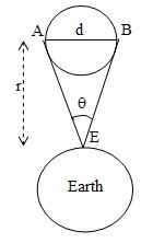
Let $\theta$ be the angle subtended by two diametrically opposite ends A and B of the moon at a point E on earth.  If r = distance of moon from earth then, $\theta =\frac{\text{ arc }}{\text{ radius }}=\frac{d}{r}$

where d is the diameter of moon

$\therefore \mathrm{d}=\mathrm{r}\times \theta$ .

ii) Parallax method: This method used to measure the distance of planets and stars from earth.

Parallactic (parallax) angle:  The angle ( $\theta$ ) subtended by the arc at the object (O) is called parallactic angle.

i.e., $\text{ Parallactic angle }=\frac{\text{ length of arc }}{\text{ radius }}$ or, $\theta =\frac{b}{s}\text{ or }s=\frac{b}{\theta }$

iii) Determination of the distances of the interior planets from the sun and the earth:  Copernicus developed a method to determine the distance of the interior planets from the earth and the sun.  Here, orbits of planets and earth around the sun are assumed to be circular.

The angle formed at the earth between the lines joining the planet and the earth and that joining the sun and the earth is known as elongation of the planet.  It is denoted by $\in$. This angle is not fixed due to orbital matrices of the planet and the earth.  Consider the state when $\angle$ SPE = 90^o.

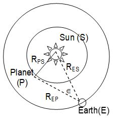
Then $\sin \in =\frac{\mathrm{PS}}{\mathrm{SE}}=\frac{{\mathrm{R}}_{\mathrm{PS}}}{{\mathrm{R}}_{\mathrm{ES}}}$

Or,  R_PS = R_ES sin $\in$

Since R_ES = 1 A.U.

$\therefore$ R_PS = (A.U.) sin $\in$ …….. (1)

Using equation (1), we can find the distance of the planet from the sun.

Also $\mathrm{cosE}=\frac{\mathrm{PE}}{\mathrm{SE}}=\frac{{\mathrm{R}}_{\mathrm{EP}}}{{\mathrm{R}}_{\mathrm{ES}}}$ Since R_ES = 1 A.U.

$\therefore$ R_EP = (A.U.) cos $\in$ ……….. (2)

Using equation (2), distance of the planet from the earth can be determined.

iv) Reflection method (Echo method):

a) RADAR (Radio Detection and Ranging):

Radar is a device to detect the aeroplane in the sky and to measure its distance from the radar station.  Radar works on the principle of reflection or echo.

Then, the distance of the aeroplane as given $\mathrm{s}=\mathrm{cx}\frac{\mathrm{t}}{2}$ , where c = speed of light.

b) SONAR (Sound Navigation and Ranging):

In this case, a strong ultrasonic wave signal from transmitter placed inside a ship is sent towards the bottom of the sea.  The signal is reflected back from the bottom of the sea and is received by the receiver in the ship.

$\therefore$ depth of the sea = d = $v\times \frac{t}{2}$ ,

where v = speed of the signal in water,  t = time after signal back to the ship.

Measurement of Mass

Mass is of two types: inertial mass and gravitational mass.

Inertial mass of a body is measured using an inertial balance.

Gravitational mass of a body is measured using a physical balance or a common balance, with which most of us are familiar.

Measurement of Time Intervals:

To measure usual time intervals, a clock is used.  Very small and very large time intervals have been measured with great accuracy.  Some techniques for measuring time intervals are given below.

i) Electrical oscillations: These use a.c. supply of frequency 50 Hz. The rotations of a synchronous motor run on a.c. is used to obtain a time scale.

ii) Electronic oscillations: A vacuum tube or a semiconductor device is used to produce electromagnetic oscillations of very high frequency. The time period of such oscillations can be used to measure small time intervals.

iii) Radioactive dating:  Very long time intervals, such as age of fossils (Carbon dating), rocks and earth etc are estimated by a technique known as radioactive dating.

22. SOME IMPORTANT PRACTICAL UNITS

1. Astronomical Unit (AU): It is the average distance of the centre of the sun from the centre of the earth. 1 AU = 1.5 x 10¹¹ m.

2. Light year (ly): One light year is the distance traveled by light in vacuum in one year. As velocity of light in vacuum is 3×10⁸ m/sec.

$\therefore$ 1 ly = 9.46×10¹⁵ m.

3. Par sec: One par sec is the distance at which an are of length 1 AU subtends an angle of 1^II 1 par sec = 3.1×10¹⁶ m = 3.26 ly.

4. Barn: Nuclear cross sections are measured in barns.

1 barn = 10^-28 m².

5. Chandrashekar limit (C.S.L): Largest practical unit of mass is C.S.L.

1 C.S.L = 1.4 times of the mass of sun.

6. Lunar month: It is the time taken by moon to compute one revolution around the earth in its orbit. 1 lunar month = 27.4 days

7. Shake: It is the smallest practical unit of time.

1 shake = 10^-8 sec.