


1. BASICS OF STATISTICS
1. STATISTICAL DATA
Statistical data are the facts which are collected for the purpose of investigation. There are two types of statistical data:
(i) Primary data: The data collected by an investigator for the first time for his own purpose are called primary data. As the primary data are collected by the user of the data, so it is more reliable and relevant.
(ii) Secondary data: The data collected by a secondary source and used by the investigator for his purpose is called secondary data. For example score of a cricket match noted from newspapers is secondary data. Thus data which are primary in the hands of one become secondary in the hands of the other. Data collected by any source also can be divided in following two types:
(i) Raw Data: Raw data are those data which are obtained from the original source but not arranged numerically. This is also called ‘ungrouped data’ for example marks of 10 students in maths are given as: 75, 96, 25, 32, 89, 62, 40, 79, 35, 55 An ‘array’ is an arrangement of raw numerical data in the ascending or descending order of magnitude. Above data can be written as 25, 32, 35, 40, 55, 62, 75, 79, 89, 96
(ii) Grouped data: An array can be placed systematically in groups or categories. For example the above data can be grouped in following manner.
| GROUPS | MARKS | TOTAL NUMBER OF STUDENTS |
| 0 to 20 | – | 0 |
| 21 to 40 | 25, 32, 35, 40 | 4 |
| 41 to 60 | 55 | 1 |
| 61 to 80 | 62, 75, 79 | 3 |
| 81 to 100 | 89, 96 | 2 |
| TOTAL | 10 | |
2. SOME BASIC DEFINITIONS
(i) Variate: Variate is a quantity that may vary from observation to observation.
(ii) Range: Range is difference between the maximum and minimum observations.
(iii) Class Interval: When data are divided in groups, each group is called a class interval.
(iv) Class Limit: Every class interval has two limits. The smallest observation of the interval is called lower limit and the largest observation of the interval is called upper limit.
(v) Class Mark: The mid value of any class is called its class mark.
(vi) Class Size: Class size is defined as the difference between two successive class marks. It is also the difference between the upper and lower limits of any class interval.
(vii) Frequency: In a particular class the count of the number of observation is called its frequency. So the corresponding frequency of a class is called its class frequency.
(viii) Cumulative Frequency: The cumulative frequency of any class is obtained by adding all the frequencies successively prior to that class i.e. it is the sum of all frequencies up to that class.
(ix) True Class Limit: In the case of exclusive classes the upper and lower limits are respectively known as its true upper limits and true lower limits. In the case of inclusive classes, the true lower and upper limits are obtained by subtracting 0.5 from the lower limit and adding 0.5 to the upper limit. True upper limits and true lower limits are also known as boundaries of the class.
(x) Tally: Tally method is used to keep the chance of error at minimum in counting. A bar (|) called tally mark is put against any item when it occurs. The fifth occurrence of any item is represented by putting diagonally a cross tally (\) on the first four tallies.
3. FREQUENCY DISTRIBUTION
The tabular arrangement of data showing the frequency of each item is called a frequency distribution table. It is a method to present raw data in the form from which one can easily understand the information contained in the raw data. Frequency distribution are of two types:
i. Discrete frequency distribution:
In this type of frequency distribution, in the first column of frequency table we write all possible values of the variables from the lowest to the highest, in the second column we write tally marks and in the third column we show frequency of each item. In this method data are not divided into groups or classes.
e.g. no. of girls in 20 families is given in following data:
1, 2, 3, 1, 1, 2, 3, 3, 4, 1, 5, 1, 1, 2, 2, 3, 3, 2, 4, 1
The above data can be put in the form of a discrete frequency distribution table in the following manner:
| S. No. | No. of girls | Tally Marks | Frequency |
| 1. | 1 | 7 | |
| 2. | 2 | 5 | |
| 3. | 3 | 5 | |
| 4. | 4 | || | 2 |
| 5. | 5 | | | 1 |
| TOTAL | 20 | ||
ii. Continuous or Grouped Frequency Distribution
In the frequency distribution data are divided into groups or classes. This method is used only where the values in the raw data are largely repeating and the difference between the greatest and the smallest observations is not very large.
4. CUMULATIVE FREQUENCY
Cumulative frequency table is obtained from the ordinary frequency table by successively adding the several frequencies. Thus to form a cumulative frequency table we add a column of cumulative frequency in the frequency distribution table. It is obvious that the cumulative frequency of the last class is the sum of the frequencies of all the classes.
Cumulative frequency series are of two types:
(i) Less than series (ii) More than series
Illustration -1
The weekly saving of 30 workers working in a factory is as given below:
64, 60, 87, 75, 69, 34, 51, 78, 39, 48, 73, 54, 63, 70, 57, 88, 90, 53, 74, 44, 31, 71, 68, 72, 36, 89, 55, 67, 73, 83
(a) Taking first class interval as 30 – 40 (40 not included), form a frequency table of equal intervals.
(b) Also form a cumulative frequency table.
(c) Find the number of workers whose weekly saving is more than Rs. 60.
Solution
(i) For the given data of the weekly saving of 30 workers working in a factory, we prepare following table:
| S. No. | Class Interval (Saving in Rs.) | Tally Marks | Frequency (No. of workers) |
| 1. | 30 – 40 | | | | | | 4 |
| 2. | 40 – 50 | | | | 2 |
| 3. | 50 – 60 | 5 | |
| 4. | 60 – 70 | 6 | |
| 5. | 70 – 80 | 8 | |
| 6. | 80 – 90 | | | | | | 4 |
| 7. | 90 – 100 | | | 1 |
| TOTAL | 30 |
(ii) For given data cumulative frequency table can be given in the following manner:
| S. No. | Class Interval (Saving in Rs.) | Tally Marks | Frequency (No. of workers) | Cumulative Frequency |
| 1. | 30 – 40 | | | | | | 4 | 4 |
| 2. | 40 – 50 | | | | 2 | 6 |
| 3. | 50 – 60 | 5 | 11 | |
| 4. | 60 – 70 | 6 | 17 | |
| 5. | 70 – 80 | 8 | 25 | |
| 6. | 80 – 90 | | | | | | 4 | 29 |
| 7. | 90 – 100 | | | 1 | 30 |
| TOTAL | 30 |
(iii) Number of workers whose weekly saving is Rs. 60 or more than Rs. 60 = (6 + 8 + 4 + 1) = 19
Illustration -2
Heights of seven persons in cm are 120, 125, 142, 134, 150, 155 and 128. Calculate the range.
Solution
For given data maximum height = 155 cm
and minimum height = 120 cm
Range = maximum height – minimum height
= 155 cm – 120 cm
= 35 cm.
Illustration -3
Form a frequency table from the following table:
| Marks | No. of Students |
| Below 10 | 15 |
| Below 20 | 35 |
| Below 30 | 60 |
| Below 40 | 84 |
| Below 50 | 96 |
| Below 60 | 127 |
| Below 70 | 198 |
| Below 80 | 250 |
Solution
For given data we make classes 0 – 10, 10 – 20, 20 – 30, ….., 70–80.
There are 15 students who obtained below 10 marks, therefore frequency of class 0 – 10 is 15. Again number of students getting below 20 marks is 35.
This includes those students also who obtained below 10 marks.
Number of students who got marks between 10 and 20 i.e. frequency of class
10 – 20 = 35–15 = 20
Thus for given data we make following table:
| S. No. | Class Interval | Comparative | Frequency |
| 1. | 0 – 10 | 15 | 15 |
| 2. | 10 – 20 | 35 | 20 |
| 3. | 20 – 30 | 60 | 25 |
| 4. | 30 – 40 | 84 | 24 |
| 5. | 40 – 50 | 96 | 12 |
| 6. | 50 – 60 | 127 | 31 |
| 7. | 60 – 70 | 198 | 71 |
| 8. | 70 – 80 | 250 | 52 |
| TOTAL | 250 |
Illustration -4
Find the unknown entries (a, b, c, d, e, f, g) from the following frequency distribution of heights of 60 students in a class:
| Height (in cm) | Frequency | Cumulative frequency |
| 160 – 165 | 15 | a |
| 165 – 170 | b | 35 |
| 170 – 175 | 12 | c |
| 175 – 180 | e | 50 |
| 180 – 185 | d | 55 |
| 185 – 190 | 5 | f |
| Total | g |
Solution
From given table, we make following cumulative frequency table:
| S. No. | Height (in cm) | Frequency | Cumulative Frequency |
| 1. | 160 – 165 | 15 | 15 = a |
| 2. | 165 – 170 | b | 15 + b = 35 |
| 3. | 170 – 175 | 12 | 15 + b + 12 = c |
| 4. | 175 – 180 | d | 15 + b + 12 + d = 50 |
| 5. | 180 – 185 | e | 15 + b + 12 + b + e = 55 |
| 6. | 185 – 190 | 5 | 15 + b + 12 + d + e + 5 = f |
| g | 60 |
Now, from table:
a = 15
15 + b = 35 b = 35 – 15 = 20
15 + b + 12 = c 15 + 20 + 12 = c
c = 47
15 + b + 12 + d = 50
15 + 20 + 12 + d = 50
d = 50 – 47
d = 3
15 + b + 12 + d + c = 55
15 + 20 + 12 + 3 + e = 55
e = 55 – 50
e = 5
15 + b + 12 + d + e + 5 = f
15 + 20 + 12 + 3 + 5 + 5 = f
f = 60
g = 60. Hence, a = 15, b = 20, c = 47, d = 3, e = 5, f = 60 and g = 60.
5. GRAPHICAL REPRESENTATION OF DATA
A given data can be represented in graphical way. There are various methods of graphical representation of frequency distribution.
(i) Bar Graphs
(ii) Histogram
(iii) Frequency Polygon
(iv) Pie Chart
Bar Graph
The frequency distribution of a discrete value is best represented by a bar graph. The height of the bars is proportional to the frequency of each variate-value. In a bar graph the bars must be kept distinct to show that the variate-values are distinct. The bars are of equal width and are drawn with equal spacing between them on the x-axis depicting the variable. The values of the variable are shown on the y-axis.
Illustration -5
The following table shows the number of illiterate persons in the age group (10–58 years) in a town:
| Age Group (in years) | 10 – 16 | 17 – 23 | 24 – 30 | 31 – 37 | 38 – 44 | 45 – 51 | 52 – 58 |
| Number of illiterate person | 175 | 375 | 100 | 150 | 250 | 400 | 525 |
Solution
Draw a bar graph to represent the above data. 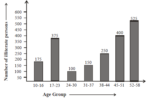
Histogram
Histogram is a graphical representation of a grouped frequency distribution with continuous classes. It consists of a set of rectangles where heights of rectangles are proportional to their class frequencies, for equal class intervals. There is no gap between two successive rectangles. The rectangles are constructed with base as the class size and their heights representing the frequencies.
Illustration -6
Construct a histogram from the following distribution of total marks obtained by 750 students of class IX in the final examination.
| Marks (mid-points) | 620 | 660 | 700 | 740 | 780 | 820 | 860 |
| Number of students | 16 | 45 | 156 | 284 | 172 | 59 | 18 |
Solution
To draw the histogram for above data first of all we find out class limits for making class intervals from given class marks.
Here difference between second and the first class marks = h = 660 – 620 = 40
lower limit of first class interval = 620 – h/2
= 620 – 20
= 600
And upper limit of the first class interval = = 620 + 20 = 640
Similarly other class intervals would be,
(660 – 20) – (660 + 20), (700 – 20) – (700 + 20), (740 – 20) – (740 + 20), (780 – 20) – (780 + 20), (820 – 20) – (820 + 20) and (860 – 20) – (860 – 20)
i.e. 640 – 680, 680 – 720, 720 – 760, 760 – 800, 800 – 840 and 840 – 880 Using these class intervals we draw following histogram taking class intervals on X-axis and number of students on Y-axis 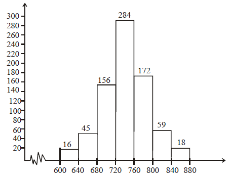
Frequency Polygon
A frequency polygon is a graph of frequency distribution. It is a line graph of class frequency which is plotted against class mark. A frequency polygon can be obtained by two methods:
(1) By using Histogram: A frequency polygon can be obtained by joining mid points of the top of the rectangles of a histogram. For this we obtain the mid points of the upper horizontal sides of each rectangle and then join these mid points by dotted lines to get frequency polygon. End of a frequency polygon preferably extended to the mid points of imagined class intervals adjacent to first and last class intervals.
Illustration -7
Draw the histogram and frequency polygon of the following frequency distribution:
| Monthly wages (in rupees) | 325-350 | 350-375 | 375-400 | 400-425 | 425-450 | Total |
| Number of workers | 30 | 45 | 75 | 60 | 55 | 245 |
Solution
Using given data we draw histogram taking monthly wages (in rupees) on X-axis and number of workers on Y-axis. Then we join the mid points of the top of the rectangles by dotted straight lines and complete it by joining the mid points of imagined class intervals adjacent to the first and last class intervals. 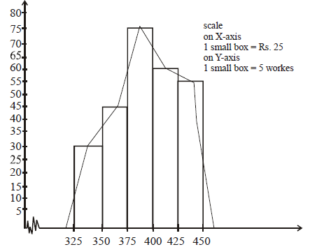
(2) Frequency polygon without using Histogram: Following procedure is used to make a frequency polygon without using histogram.
(i) Calculate the class marks, x1, x2, …., xn of each of the given class intervals.
(ii) Mark class marks x1, x2, …., xn, along X-axis and frequencies f1, f2, …. fn along Y-axis.
(iii) Plot the points (x1, f1), (x2, f2), ,….., (xn, fn).
(iv) Obtain the mid-points of two class intervals of zero frequencies at the beginning of the first interval and at the end of the last interval.
(v) Join the points (x1, f1), (x2, f2), …, (xn, fn) by the line segments and complete the frequency polygon by joining the mid points of the first and last intervals to the mid points of the imagined classes adjacent to them.
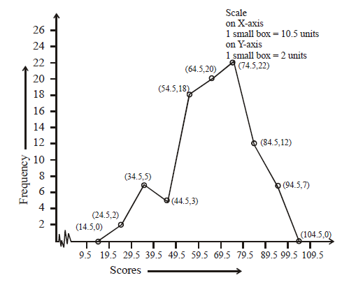
Illustration -8
Represent the following distribution by a frequency polygon without using a histogram:
| Scores | 20-29 | 30-39 | 40-49 | 50-59 | 60-69 | 70-79 | 80-89 | 90-99 |
| Frequency | 2 | 5 | 3 | 18 | 20 | 22 | 12 | 7 |
Solution
Given data is in the form of inclusive classes, so first of all we shall convert them into exclusive classes. Also we have to get class marks of these class intervals for this purpose.
| S. No. | Scores | True Class Limits | Class Marks | Frequency | Points to be plotted |
| 1. | 20 – 29 | 19.5 – 29.5 | 24.5 | 2 | (24.5, 2) |
| 2. | 30 – 39 | 29.5 – 39.5 | 34.5 | 5 | (34.5, 5) |
| 3. | 40 – 49 | 39.5 – 49.5 | 44.5 | 3 | (44.5, 3) |
| 4. | 50 – 59 | 49.5 – 59.5 | 54.5 | 18 | (54.5, 18) |
| 5. | 60 – 69 | 59.5 – 69.5 | 64.5 | 20 | (64.5, 20) |
| 6. | 70 – 79 | 69.5 – 79.5 | 74.5 | 22 | (74.5, 22) |
| 7. | 80 – 89 | 79.5 – 89.5 | 84.5 | 12 | (84.5, 12) |
| 8. | 90 – 99 | 89.5 – 99.5 | 94.5 | 7 | (94.5, 7) |
Plotting these points and joining them by line segments we get frequency polygon. We complete the frequency polygon by extending it up to points (14.5, 0) and (104.5, 0) adjacent to first and last class marks on X-axis.
Pie Chart
In a pie-chart, various observations or components are represented by the sectors of a circle and the whole circle represents the sum of the values of all the components. Clearly, the total angle of 360o at the center of the circle is divided according to the values of the components. Thus we have, Central Angle for Component
=
Sometimes, the value of components are expressed in percentages. In such cases, we have: Central Angle for Component =
Illustration -9
A survey was conducted among a group of girls to know their preferences for the types of slippers. The given circle graph shows the results of the survey.
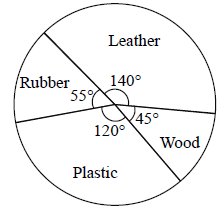
If the survey was conducted among a group of 1080 girls, then find out how many girls preferred to wear leather slippers?
(A) 140 (B) 280 (C) 420 (D) 560
Solution
C
In the given circle graph, it is seen that the central angle of the sector corresponding to leather slippers is 140°.
Therefore, number of girls who preferred to wear leather slippers:
Thus, 420 girls preferred to wear leather slippers.
6. MEASURES OF CENTRAL TENDENCY
One of the most important objectives of statistical analysis is to get one single value that describes the characteristic of the entire data. Such a value is called the central value or an average. The following are the important types of averages:
1. Arithmetic Mean
2. Geometric Mean
3. Harmonic mean
4. Median
5. Mode
We consider these measures in three cases (i) Individual series (i.e. each individual observation is given) (ii) discrete series (i.e., the observations along with number of times a particular observation called the frequency is given) (iii) continuous series (i.e. the class intervals along with their frequencies are given)
2. Arithmetic Mean
The average of numbers in arithmetic is known as the Arithmetic Mean of these numbers in statistics.
1. MEAN OF AN UNGROUPED DATA
The Arithmetic Mean or simply the Mean of n observations x1, x2, x3, …….xn is given by the formula:
Mean =
Where the symbol , called sigma stands for the summation of the terms.
Illustration -10
Calculate the mean of the following numbers: 3, 1, 5, 6, 3, 4, 5, 3, 7, 2
Solution
Sum of the given numbers = (3 + 1 + 5 + 6 + 3 + 4 + 5 + 3 + 7 + 2) = 39.
Number of these numbers = 10.
Mean of the given numbers = .
Illustration -11
The weights (in kg) of 5 persons in a group are: 55, 63, 48, 59 and 61. Find their mean weight.
Solution
Sum of the weight of all persons = (55 + 63 + 48 + 59 + 61) kg = 286 kg.
Number of persons = 5.
Mean weight = kg = 57.2 kg.
Some Useful Result: Let the mean of x1 x2 x3, ……..xn be A. Then
(i) Mean of (x1 + k), (x2 + k), (x3+ k) ………..(xn + k) is (A + k);
(ii) Mean of (x1 – k), (x2 – k), (x3 – k)………..(xn – k) is (A – k);
(iii) Mean of kx1, kx2, kx3 …….. kxn is kA, where k 0.
2. MEAN OF GROUPED DATA
Direct Method
When the variates x1, x2, x3, …………xn have frequencies f1, f2, f3 ……..fn respectively, then the mean is given by the formula:
Mean = .
Illustration -12
The following table shows the weights of 15 members of an athletic team in a school.
| Weight (in kg) | 42 | 45 | 46 | 48 | 49 |
| Number of athletes | 4 | 3 | 5 | 2 | 1 |
Find the mean weight.
Solution
From the above data, we may prepare the table given below.
|
Weight (in kg) xi |
Number of athletes (Frequency) |
|
|
42 45 46 48 49 |
4 3 5 2 1 |
168 135 230 96 49 |
|
|
= 15 |
= 678 |
Mean Weight =.
Illustration -13
Using short cut method, calculate the mean weekly wage from the following frequency distribution.
| Weekly wages(in Rs) | 950 | 1000 | 1050 | 1100 | 1250 | 1500 | 1600 |
| Number of workers | 24 | 18 | 13 | 15 | 20 | 11 | 9 |
Solution
Let the assumed mean be, A = 1100.
From the given data, we may prepare the table given below.
|
Weekly Wages (in Rs) x1 |
Numbers of Workers (Frequency) |
di = (xi – A) = (xi – 1100) |
fidi |
|
950 1000 1050 1100 = A 1250 1500 1600 |
24 18 13 15 20 11 9 |
–150 –100 –50 0 150 400 500 |
–3600 –1800 –650 0 3000 4400 4500 |
|
|
fI = 110 |
|
fI di = 5850 |
Mean =
Hence, Mean Wage = Rs 1153.18.
3. MEAN OF GROUPED DATA IN THE FORM OF CLASSES
I. Direct Method
Step 1: For each class, find the class mark xi by using the relation, xi = (lower limit + upper limit). Step 2: Use the formula, Mean = .
II. Short Cut Method or Deviation Method
Step 1: For each class, find the class mark xi.
Step 2: Let A be the assumed mean.
Step 3: Find di = (xi – A).
Step 4: Use the formula, Mean = .
III. Step-Deviation Method
Step 1. For each class, find the class mark x1.
Step 2: Let A be the assumed mean.
Step 3: Calculate, , where c is the class size.
Step 4: Use the formula, Mean = .
Illustration -14
Using direct method, find the mean of the following frequency distribution:
| Class-interval | 10-20 | 20-30 | 30-40 | 40-50 | 50-60 | 60-70 |
| Frequency | 6 | 8 | 12 | 15 | 10 | 9 |
Solution
From the given data, we may prepare the table given below.
|
Class-Interval |
Class-Mark xi |
Frequency fi |
fixi |
|
10-20 20-30 30-40 40-50 50-60 60-70 |
15 25 35 45 55 65 |
6 8 12 15 10 9 |
90 200 420 675 550 585 |
|
|
|
fI = 60 |
fixi = 2520 |
Mean = .
Illustration -15
Using Short Cut Method find the mean for the following frequency distribution:
| Class-interval | 84-90 | 90-96 | 96-102 | 102-108 | 108-114 | 114-120 |
| Frequency | 8 | 10 | 16 | 23 | 12 | 11 |
Solution
From the given data, we may prepare the table given below.
|
Class-Interval |
Class-Mark xi |
Frequency fi |
di = (xi – A) = (xi – 99) |
fidi |
|
84-90 90-96 96-102 102-108 108-114 114-120 |
87 93 99 = A 105 111 117 |
8 10 16 23 12 11 |
–12 –6 0 6 12 18 |
–96 –60 0 138 144 198 |
|
|
|
fI = 80 |
|
fidi = 324 |
Mean =
Hence, Mean = 103.05.
Illustration -16
Using Step Deviation Method, calculate the mean for the following data:
| Height (in cm) | 135-140 | 140-145 | 145-150 | 150-155 | 155-160 | 160-165 | 165-170 | 170-175 |
| Frequency | 4 | 9 | 18 | 28 | 24 | 10 | 5 | 2 |
Solution
Here, class size, c = 5. Take assumed mean, A = 152.5. Thus, from the given data, we may prepare
|
Class-Interval |
Class-Mark xi |
Frequency fi |
fii |
|
|
135-140 140-145 145-150 150-155 155-160 160-165 165-170 170-175- |
137.5 142.5 147.5 152.5 = A 157.5 162.5 167.5 172.5 |
4 9 18 28 24 10 5 2 |
–3 –2 –1 0 1 2 3 4 |
–12 –18 –18 0 24 20 15 8 |
|
|
|
fI = 100 |
|
fii = 19 |
Mean = = (152.5 + 0.95) = 153.45 cm.
4. IMPORTANT FORMULAE FOR SOLVING ARITHMETIC MEAN
1. Arithmetic Mean of Individual Series
If x1, x2 , x3,….., xn are n values of variant x, then its Arithmetic Mean, denoted by x is
(or)
where A is the assumed average. (For individual series)
2. Arithmetic Mean of Discreate Series
If a variable takes values x1, x2 , x3,….., xn with corresponding frequencies f1, f2 , f3,….., fn then the arithmetic mean is given by
where
3. Arithmetic Mean Of Continuous Series
In case of a set of data with class intervals, we cannot find the exact value of the mean because we do not know the exact values of the variables. We, therefore, try to obtain an approximate value of the mean. The method of approximate is to replace all the observed values belonging to a class by mid-value of the class.
If x1, x2 , x3,….., xn are the mid values of the class intervals having corresponding frequencies f1, f2 , f3,….., fn then we apply the same formula as in discrete series.
4. Combined Arithmetic Mean
If are the means of k – series of sizes then the combined or composite mean can be obtained by the formula :
5. Weighted Arithmetic Mean
If w1, w2 , w3,….., wn be the weights assigned to the values x1, x2 , x3,….., xn be respectively of a variable x, then the weighted A.M. is .
5. PROPERTIES OF ARITHMETIC MEAN
1. Sum of all the deviations from arithmetic mean is zero i.e.,
(in case of individual series)
(in case of discrete or continuous series)
2. If each observation is increased or decreased by a given constant K, the mean is also increased or decreased by K
The property is also known as effect of change of origin. K can be taken to be any number. However, to simplify the calculations, K should be taken as a value which is in the middle of the table.
3. Step Deviation Method or change of scale
If x1, x2 , x3,….., xn are mid values of class intervals with corresponding frequencies f1, f2 , f3,….., fn then we may change the scale by taking in this case.
(if A is assumed mean)
A and h can be any numbers but if the lengths of class intervals are equal then h may be taken as width of the class interval.
In particular if each observation is multiplied or divided by a constant, the mean is also multiplied or divided by the same constant.
4. The sum of the squared deviation of the variate from their mean is minimum i.e., the quantity is minimum when .
5. E(aX + b) = aE(X) + b (where E(X) = Mean of X)
Illustration-17
The weighted mean of the first n natural numbers, the weights being the corresponding numbers, is
Solution
First n natural numbers are 1, 2, 3,…,n; whose corresponding weights are 1, 2, 3,…,n respectively.
weight mean =
Illustration-18
The weighted mean of the first n natural numbers whose weights are equal to the squares of the corresponding numbers is
Solution
weighted mean =
Illustration-19
The average salary of male employees in a firm is Rs. 5200 and that of females is Rs.4200. The mean salary of all the employees is Rs.5000. The percentage of male and female employees are respectively is
Solution
Let
Also, we know that
The percentage of male employees in the firm =
and the percentage of female employees in the firm =
Illustration-20
If the mean of 9 observations is 100 and mean of 6 observations is 80, then the mean of 15 observations is
Solution
1. BASICS OF STATISTICS
1. STATISTICAL DATA
Statistical data are the facts which are collected for the purpose of investigation. There are two types of statistical data:
(i) Primary data: The data collected by an investigator for the first time for his own purpose are called primary data. As the primary data are collected by the user of the data, so it is more reliable and relevant.
(ii) Secondary data: The data collected by a secondary source and used by the investigator for his purpose is called secondary data. For example score of a cricket match noted from newspapers is secondary data. Thus data which are primary in the hands of one become secondary in the hands of the other. Data collected by any source also can be divided in following two types:
(i) Raw Data: Raw data are those data which are obtained from the original source but not arranged numerically. This is also called ‘ungrouped data’ for example marks of 10 students in maths are given as: 75, 96, 25, 32, 89, 62, 40, 79, 35, 55 An ‘array’ is an arrangement of raw numerical data in the ascending or descending order of magnitude. Above data can be written as 25, 32, 35, 40, 55, 62, 75, 79, 89, 96
(ii) Grouped data: An array can be placed systematically in groups or categories. For example the above data can be grouped in following manner.
| GROUPS | MARKS | TOTAL NUMBER OF STUDENTS |
| 0 to 20 | – | 0 |
| 21 to 40 | 25, 32, 35, 40 | 4 |
| 41 to 60 | 55 | 1 |
| 61 to 80 | 62, 75, 79 | 3 |
| 81 to 100 | 89, 96 | 2 |
| TOTAL | 10 | |
2. SOME BASIC DEFINITIONS
(i) Variate: Variate is a quantity that may vary from observation to observation.
(ii) Range: Range is difference between the maximum and minimum observations.
(iii) Class Interval: When data are divided in groups, each group is called a class interval.
(iv) Class Limit: Every class interval has two limits. The smallest observation of the interval is called lower limit and the largest observation of the interval is called upper limit.
(v) Class Mark: The mid value of any class is called its class mark.
(vi) Class Size: Class size is defined as the difference between two successive class marks. It is also the difference between the upper and lower limits of any class interval.
(vii) Frequency: In a particular class the count of the number of observation is called its frequency. So the corresponding frequency of a class is called its class frequency.
(viii) Cumulative Frequency: The cumulative frequency of any class is obtained by adding all the frequencies successively prior to that class i.e. it is the sum of all frequencies up to that class.
(ix) True Class Limit: In the case of exclusive classes the upper and lower limits are respectively known as its true upper limits and true lower limits. In the case of inclusive classes, the true lower and upper limits are obtained by subtracting 0.5 from the lower limit and adding 0.5 to the upper limit. True upper limits and true lower limits are also known as boundaries of the class.
(x) Tally: Tally method is used to keep the chance of error at minimum in counting. A bar (|) called tally mark is put against any item when it occurs. The fifth occurrence of any item is represented by putting diagonally a cross tally (\) on the first four tallies.
3. FREQUENCY DISTRIBUTION
The tabular arrangement of data showing the frequency of each item is called a frequency distribution table. It is a method to present raw data in the form from which one can easily understand the information contained in the raw data. Frequency distribution are of two types:
i. Discrete frequency distribution:
In this type of frequency distribution, in the first column of frequency table we write all possible values of the variables from the lowest to the highest, in the second column we write tally marks and in the third column we show frequency of each item. In this method data are not divided into groups or classes.
e.g. no. of girls in 20 families is given in following data:
1, 2, 3, 1, 1, 2, 3, 3, 4, 1, 5, 1, 1, 2, 2, 3, 3, 2, 4, 1
The above data can be put in the form of a discrete frequency distribution table in the following manner:
| S. No. | No. of girls | Tally Marks | Frequency |
| 1. | 1 | 7 | |
| 2. | 2 | 5 | |
| 3. | 3 | 5 | |
| 4. | 4 | || | 2 |
| 5. | 5 | | | 1 |
| TOTAL | 20 | ||
ii. Continuous or Grouped Frequency Distribution
In the frequency distribution data are divided into groups or classes. This method is used only where the values in the raw data are largely repeating and the difference between the greatest and the smallest observations is not very large.
4. CUMULATIVE FREQUENCY
Cumulative frequency table is obtained from the ordinary frequency table by successively adding the several frequencies. Thus to form a cumulative frequency table we add a column of cumulative frequency in the frequency distribution table. It is obvious that the cumulative frequency of the last class is the sum of the frequencies of all the classes.
Cumulative frequency series are of two types:
(i) Less than series (ii) More than series
Illustration -1
The weekly saving of 30 workers working in a factory is as given below:
64, 60, 87, 75, 69, 34, 51, 78, 39, 48, 73, 54, 63, 70, 57, 88, 90, 53, 74, 44, 31, 71, 68, 72, 36, 89, 55, 67, 73, 83
(a) Taking first class interval as 30 – 40 (40 not included), form a frequency table of equal intervals.
(b) Also form a cumulative frequency table.
(c) Find the number of workers whose weekly saving is more than Rs. 60.
Solution
(i) For the given data of the weekly saving of 30 workers working in a factory, we prepare following table:
| S. No. | Class Interval (Saving in Rs.) | Tally Marks | Frequency (No. of workers) |
| 1. | 30 – 40 | | | | | | 4 |
| 2. | 40 – 50 | | | | 2 |
| 3. | 50 – 60 | 5 | |
| 4. | 60 – 70 | 6 | |
| 5. | 70 – 80 | 8 | |
| 6. | 80 – 90 | | | | | | 4 |
| 7. | 90 – 100 | | | 1 |
| TOTAL | 30 |
(ii) For given data cumulative frequency table can be given in the following manner:
| S. No. | Class Interval (Saving in Rs.) | Tally Marks | Frequency (No. of workers) | Cumulative Frequency |
| 1. | 30 – 40 | | | | | | 4 | 4 |
| 2. | 40 – 50 | | | | 2 | 6 |
| 3. | 50 – 60 | 5 | 11 | |
| 4. | 60 – 70 | 6 | 17 | |
| 5. | 70 – 80 | 8 | 25 | |
| 6. | 80 – 90 | | | | | | 4 | 29 |
| 7. | 90 – 100 | | | 1 | 30 |
| TOTAL | 30 |
(iii) Number of workers whose weekly saving is Rs. 60 or more than Rs. 60 = (6 + 8 + 4 + 1) = 19
Illustration -2
Heights of seven persons in cm are 120, 125, 142, 134, 150, 155 and 128. Calculate the range.
Solution
For given data maximum height = 155 cm
and minimum height = 120 cm
Range = maximum height – minimum height
= 155 cm – 120 cm
= 35 cm.
Illustration -3
Form a frequency table from the following table:
| Marks | No. of Students |
| Below 10 | 15 |
| Below 20 | 35 |
| Below 30 | 60 |
| Below 40 | 84 |
| Below 50 | 96 |
| Below 60 | 127 |
| Below 70 | 198 |
| Below 80 | 250 |
Solution
For given data we make classes 0 – 10, 10 – 20, 20 – 30, ….., 70–80.
There are 15 students who obtained below 10 marks, therefore frequency of class 0 – 10 is 15. Again number of students getting below 20 marks is 35.
This includes those students also who obtained below 10 marks.
Number of students who got marks between 10 and 20 i.e. frequency of class
10 – 20 = 35–15 = 20
Thus for given data we make following table:
| S. No. | Class Interval | Comparative | Frequency |
| 1. | 0 – 10 | 15 | 15 |
| 2. | 10 – 20 | 35 | 20 |
| 3. | 20 – 30 | 60 | 25 |
| 4. | 30 – 40 | 84 | 24 |
| 5. | 40 – 50 | 96 | 12 |
| 6. | 50 – 60 | 127 | 31 |
| 7. | 60 – 70 | 198 | 71 |
| 8. | 70 – 80 | 250 | 52 |
| TOTAL | 250 |
Illustration -4
Find the unknown entries (a, b, c, d, e, f, g) from the following frequency distribution of heights of 60 students in a class:
| Height (in cm) | Frequency | Cumulative frequency |
| 160 – 165 | 15 | a |
| 165 – 170 | b | 35 |
| 170 – 175 | 12 | c |
| 175 – 180 | e | 50 |
| 180 – 185 | d | 55 |
| 185 – 190 | 5 | f |
| Total | g |
Solution
From given table, we make following cumulative frequency table:
| S. No. | Height (in cm) | Frequency | Cumulative Frequency |
| 1. | 160 – 165 | 15 | 15 = a |
| 2. | 165 – 170 | b | 15 + b = 35 |
| 3. | 170 – 175 | 12 | 15 + b + 12 = c |
| 4. | 175 – 180 | d | 15 + b + 12 + d = 50 |
| 5. | 180 – 185 | e | 15 + b + 12 + b + e = 55 |
| 6. | 185 – 190 | 5 | 15 + b + 12 + d + e + 5 = f |
| g | 60 |
Now, from table:
a = 15
15 + b = 35 b = 35 – 15 = 20
15 + b + 12 = c 15 + 20 + 12 = c
c = 47
15 + b + 12 + d = 50
15 + 20 + 12 + d = 50
d = 50 – 47
d = 3
15 + b + 12 + d + c = 55
15 + 20 + 12 + 3 + e = 55
e = 55 – 50
e = 5
15 + b + 12 + d + e + 5 = f
15 + 20 + 12 + 3 + 5 + 5 = f
f = 60
g = 60. Hence, a = 15, b = 20, c = 47, d = 3, e = 5, f = 60 and g = 60.
5. GRAPHICAL REPRESENTATION OF DATA
A given data can be represented in graphical way. There are various methods of graphical representation of frequency distribution.
(i) Bar Graphs
(ii) Histogram
(iii) Frequency Polygon
(iv) Pie Chart
Bar Graph
The frequency distribution of a discrete value is best represented by a bar graph. The height of the bars is proportional to the frequency of each variate-value. In a bar graph the bars must be kept distinct to show that the variate-values are distinct. The bars are of equal width and are drawn with equal spacing between them on the x-axis depicting the variable. The values of the variable are shown on the y-axis.
Illustration -5
The following table shows the number of illiterate persons in the age group (10–58 years) in a town:
| Age Group (in years) | 10 – 16 | 17 – 23 | 24 – 30 | 31 – 37 | 38 – 44 | 45 – 51 | 52 – 58 |
| Number of illiterate person | 175 | 375 | 100 | 150 | 250 | 400 | 525 |
Solution
Draw a bar graph to represent the above data.
Histogram
Histogram is a graphical representation of a grouped frequency distribution with continuous classes. It consists of a set of rectangles where heights of rectangles are proportional to their class frequencies, for equal class intervals. There is no gap between two successive rectangles. The rectangles are constructed with base as the class size and their heights representing the frequencies.
Illustration -6
Construct a histogram from the following distribution of total marks obtained by 750 students of class IX in the final examination.
| Marks (mid-points) | 620 | 660 | 700 | 740 | 780 | 820 | 860 |
| Number of students | 16 | 45 | 156 | 284 | 172 | 59 | 18 |
Solution
To draw the histogram for above data first of all we find out class limits for making class intervals from given class marks.
Here difference between second and the first class marks = h = 660 – 620 = 40
lower limit of first class interval = 620 – h/2
= 620 – 20
= 600
And upper limit of the first class interval = = 620 + 20 = 640
Similarly other class intervals would be,
(660 – 20) – (660 + 20), (700 – 20) – (700 + 20), (740 – 20) – (740 + 20), (780 – 20) – (780 + 20), (820 – 20) – (820 + 20) and (860 – 20) – (860 – 20)
i.e. 640 – 680, 680 – 720, 720 – 760, 760 – 800, 800 – 840 and 840 – 880 Using these class intervals we draw following histogram taking class intervals on X-axis and number of students on Y-axis
Frequency Polygon
A frequency polygon is a graph of frequency distribution. It is a line graph of class frequency which is plotted against class mark. A frequency polygon can be obtained by two methods:
(1) By using Histogram: A frequency polygon can be obtained by joining mid points of the top of the rectangles of a histogram. For this we obtain the mid points of the upper horizontal sides of each rectangle and then join these mid points by dotted lines to get frequency polygon. End of a frequency polygon preferably extended to the mid points of imagined class intervals adjacent to first and last class intervals.
Illustration -7
Draw the histogram and frequency polygon of the following frequency distribution:
| Monthly wages (in rupees) | 325-350 | 350-375 | 375-400 | 400-425 | 425-450 | Total |
| Number of workers | 30 | 45 | 75 | 60 | 55 | 245 |
Solution
Using given data we draw histogram taking monthly wages (in rupees) on X-axis and number of workers on Y-axis. Then we join the mid points of the top of the rectangles by dotted straight lines and complete it by joining the mid points of imagined class intervals adjacent to the first and last class intervals.
(2) Frequency polygon without using Histogram: Following procedure is used to make a frequency polygon without using histogram.
(i) Calculate the class marks, x1, x2, …., xn of each of the given class intervals.
(ii) Mark class marks x1, x2, …., xn, along X-axis and frequencies f1, f2, …. fn along Y-axis.
(iii) Plot the points (x1, f1), (x2, f2), ,….., (xn, fn).
(iv) Obtain the mid-points of two class intervals of zero frequencies at the beginning of the first interval and at the end of the last interval.
(v) Join the points (x1, f1), (x2, f2), …, (xn, fn) by the line segments and complete the frequency polygon by joining the mid points of the first and last intervals to the mid points of the imagined classes adjacent to them.
Illustration -8
Represent the following distribution by a frequency polygon without using a histogram:
| Scores | 20-29 | 30-39 | 40-49 | 50-59 | 60-69 | 70-79 | 80-89 | 90-99 |
| Frequency | 2 | 5 | 3 | 18 | 20 | 22 | 12 | 7 |
Solution
Given data is in the form of inclusive classes, so first of all we shall convert them into exclusive classes. Also we have to get class marks of these class intervals for this purpose.
| S. No. | Scores | True Class Limits | Class Marks | Frequency | Points to be plotted |
| 1. | 20 – 29 | 19.5 – 29.5 | 24.5 | 2 | (24.5, 2) |
| 2. | 30 – 39 | 29.5 – 39.5 | 34.5 | 5 | (34.5, 5) |
| 3. | 40 – 49 | 39.5 – 49.5 | 44.5 | 3 | (44.5, 3) |
| 4. | 50 – 59 | 49.5 – 59.5 | 54.5 | 18 | (54.5, 18) |
| 5. | 60 – 69 | 59.5 – 69.5 | 64.5 | 20 | (64.5, 20) |
| 6. | 70 – 79 | 69.5 – 79.5 | 74.5 | 22 | (74.5, 22) |
| 7. | 80 – 89 | 79.5 – 89.5 | 84.5 | 12 | (84.5, 12) |
| 8. | 90 – 99 | 89.5 – 99.5 | 94.5 | 7 | (94.5, 7) |
Plotting these points and joining them by line segments we get frequency polygon. We complete the frequency polygon by extending it up to points (14.5, 0) and (104.5, 0) adjacent to first and last class marks on X-axis.
Pie Chart
In a pie-chart, various observations or components are represented by the sectors of a circle and the whole circle represents the sum of the values of all the components. Clearly, the total angle of 360o at the center of the circle is divided according to the values of the components. Thus we have, Central Angle for Component
=
Sometimes, the value of components are expressed in percentages. In such cases, we have: Central Angle for Component =
Illustration -9
A survey was conducted among a group of girls to know their preferences for the types of slippers. The given circle graph shows the results of the survey.
If the survey was conducted among a group of 1080 girls, then find out how many girls preferred to wear leather slippers?
(A) 140 (B) 280 (C) 420 (D) 560
Solution
C
In the given circle graph, it is seen that the central angle of the sector corresponding to leather slippers is 140°.
Therefore, number of girls who preferred to wear leather slippers:
Thus, 420 girls preferred to wear leather slippers.
6. MEASURES OF CENTRAL TENDENCY
One of the most important objectives of statistical analysis is to get one single value that describes the characteristic of the entire data. Such a value is called the central value or an average. The following are the important types of averages:
1. Arithmetic Mean
2. Geometric Mean
3. Harmonic mean
4. Median
5. Mode
We consider these measures in three cases (i) Individual series (i.e. each individual observation is given) (ii) discrete series (i.e., the observations along with number of times a particular observation called the frequency is given) (iii) continuous series (i.e. the class intervals along with their frequencies are given)
2. Arithmetic Mean
The average of numbers in arithmetic is known as the Arithmetic Mean of these numbers in statistics.
1. MEAN OF AN UNGROUPED DATA
The Arithmetic Mean or simply the Mean of n observations x1, x2, x3, …….xn is given by the formula:
Mean =
Where the symbol , called sigma stands for the summation of the terms.
Illustration -10
Calculate the mean of the following numbers: 3, 1, 5, 6, 3, 4, 5, 3, 7, 2
Solution
Sum of the given numbers = (3 + 1 + 5 + 6 + 3 + 4 + 5 + 3 + 7 + 2) = 39.
Number of these numbers = 10.
Mean of the given numbers = .
Illustration -11
The weights (in kg) of 5 persons in a group are: 55, 63, 48, 59 and 61. Find their mean weight.
Solution
Sum of the weight of all persons = (55 + 63 + 48 + 59 + 61) kg = 286 kg.
Number of persons = 5.
Mean weight = kg = 57.2 kg.
Some Useful Result: Let the mean of x1 x2 x3, ……..xn be A. Then
(i) Mean of (x1 + k), (x2 + k), (x3+ k) ………..(xn + k) is (A + k);
(ii) Mean of (x1 – k), (x2 – k), (x3 – k)………..(xn – k) is (A – k);
(iii) Mean of kx1, kx2, kx3 …….. kxn is kA, where k 0.
2. MEAN OF GROUPED DATA
Direct Method
When the variates x1, x2, x3, …………xn have frequencies f1, f2, f3 ……..fn respectively, then the mean is given by the formula:
Mean = .
Illustration -12
The following table shows the weights of 15 members of an athletic team in a school.
| Weight (in kg) | 42 | 45 | 46 | 48 | 49 |
| Number of athletes | 4 | 3 | 5 | 2 | 1 |
Find the mean weight.
Solution
From the above data, we may prepare the table given below.
|
Weight (in kg) xi |
Number of athletes (Frequency) |
|
|
42 45 46 48 49 |
4 3 5 2 1 |
168 135 230 96 49 |
|
|
= 15 |
= 678 |
Mean Weight =.
Illustration -13
Using short cut method, calculate the mean weekly wage from the following frequency distribution.
| Weekly wages(in Rs) | 950 | 1000 | 1050 | 1100 | 1250 | 1500 | 1600 |
| Number of workers | 24 | 18 | 13 | 15 | 20 | 11 | 9 |
Solution
Let the assumed mean be, A = 1100.
From the given data, we may prepare the table given below.
|
Weekly Wages (in Rs) x1 |
Numbers of Workers (Frequency) |
di = (xi – A) = (xi – 1100) |
fidi |
|
950 1000 1050 1100 = A 1250 1500 1600 |
24 18 13 15 20 11 9 |
–150 –100 –50 0 150 400 500 |
–3600 –1800 –650 0 3000 4400 4500 |
|
|
fI = 110 |
|
fI di = 5850 |
Mean =
Hence, Mean Wage = Rs 1153.18.
3. MEAN OF GROUPED DATA IN THE FORM OF CLASSES
I. Direct Method
Step 1: For each class, find the class mark xi by using the relation, xi = (lower limit + upper limit). Step 2: Use the formula, Mean = .
II. Short Cut Method or Deviation Method
Step 1: For each class, find the class mark xi.
Step 2: Let A be the assumed mean.
Step 3: Find di = (xi – A).
Step 4: Use the formula, Mean = .
III. Step-Deviation Method
Step 1. For each class, find the class mark x1.
Step 2: Let A be the assumed mean.
Step 3: Calculate, , where c is the class size.
Step 4: Use the formula, Mean = .
Illustration -14
Using direct method, find the mean of the following frequency distribution:
| Class-interval | 10-20 | 20-30 | 30-40 | 40-50 | 50-60 | 60-70 |
| Frequency | 6 | 8 | 12 | 15 | 10 | 9 |
Solution
From the given data, we may prepare the table given below.
|
Class-Interval |
Class-Mark xi |
Frequency fi |
fixi |
|
10-20 20-30 30-40 40-50 50-60 60-70 |
15 25 35 45 55 65 |
6 8 12 15 10 9 |
90 200 420 675 550 585 |
|
|
|
fI = 60 |
fixi = 2520 |
Mean = .
Illustration -15
Using Short Cut Method find the mean for the following frequency distribution:
| Class-interval | 84-90 | 90-96 | 96-102 | 102-108 | 108-114 | 114-120 |
| Frequency | 8 | 10 | 16 | 23 | 12 | 11 |
Solution
From the given data, we may prepare the table given below.
|
Class-Interval |
Class-Mark xi |
Frequency fi |
di = (xi – A) = (xi – 99) |
fidi |
|
84-90 90-96 96-102 102-108 108-114 114-120 |
87 93 99 = A 105 111 117 |
8 10 16 23 12 11 |
–12 –6 0 6 12 18 |
–96 –60 0 138 144 198 |
|
|
|
fI = 80 |
|
fidi = 324 |
Mean =
Hence, Mean = 103.05.
Illustration -16
Using Step Deviation Method, calculate the mean for the following data:
| Height (in cm) | 135-140 | 140-145 | 145-150 | 150-155 | 155-160 | 160-165 | 165-170 | 170-175 |
| Frequency | 4 | 9 | 18 | 28 | 24 | 10 | 5 | 2 |
Solution
Here, class size, c = 5. Take assumed mean, A = 152.5. Thus, from the given data, we may prepare
|
Class-Interval |
Class-Mark xi |
Frequency fi |
fii |
|
|
135-140 140-145 145-150 150-155 155-160 160-165 165-170 170-175- |
137.5 142.5 147.5 152.5 = A 157.5 162.5 167.5 172.5 |
4 9 18 28 24 10 5 2 |
–3 –2 –1 0 1 2 3 4 |
–12 –18 –18 0 24 20 15 8 |
|
|
|
fI = 100 |
|
fii = 19 |
Mean = = (152.5 + 0.95) = 153.45 cm.
4. IMPORTANT FORMULAE FOR SOLVING ARITHMETIC MEAN
1. Arithmetic Mean of Individual Series
If x1, x2 , x3,….., xn are n values of variant x, then its Arithmetic Mean, denoted by x is
(or)
where A is the assumed average. (For individual series)
2. Arithmetic Mean of Discreate Series
If a variable takes values x1, x2 , x3,….., xn with corresponding frequencies f1, f2 , f3,….., fn then the arithmetic mean is given by
where
3. Arithmetic Mean Of Continuous Series
In case of a set of data with class intervals, we cannot find the exact value of the mean because we do not know the exact values of the variables. We, therefore, try to obtain an approximate value of the mean. The method of approximate is to replace all the observed values belonging to a class by mid-value of the class.
If x1, x2 , x3,….., xn are the mid values of the class intervals having corresponding frequencies f1, f2 , f3,….., fn then we apply the same formula as in discrete series.
4. Combined Arithmetic Mean
If are the means of k – series of sizes then the combined or composite mean can be obtained by the formula :
5. Weighted Arithmetic Mean
If w1, w2 , w3,….., wn be the weights assigned to the values x1, x2 , x3,….., xn be respectively of a variable x, then the weighted A.M. is .
5. PROPERTIES OF ARITHMETIC MEAN
1. Sum of all the deviations from arithmetic mean is zero i.e.,
(in case of individual series)
(in case of discrete or continuous series)
2. If each observation is increased or decreased by a given constant K, the mean is also increased or decreased by K
The property is also known as effect of change of origin. K can be taken to be any number. However, to simplify the calculations, K should be taken as a value which is in the middle of the table.
3. Step Deviation Method or change of scale
If x1, x2 , x3,….., xn are mid values of class intervals with corresponding frequencies f1, f2 , f3,….., fn then we may change the scale by taking in this case.
(if A is assumed mean)
A and h can be any numbers but if the lengths of class intervals are equal then h may be taken as width of the class interval.
In particular if each observation is multiplied or divided by a constant, the mean is also multiplied or divided by the same constant.
4. The sum of the squared deviation of the variate from their mean is minimum i.e., the quantity is minimum when .
5. E(aX + b) = aE(X) + b (where E(X) = Mean of X)
Illustration-17
The weighted mean of the first n natural numbers, the weights being the corresponding numbers, is
Solution
First n natural numbers are 1, 2, 3,…,n; whose corresponding weights are 1, 2, 3,…,n respectively.
weight mean =
Illustration-18
The weighted mean of the first n natural numbers whose weights are equal to the squares of the corresponding numbers is
Solution
weighted mean =
Illustration-19
The average salary of male employees in a firm is Rs. 5200 and that of females is Rs.4200. The mean salary of all the employees is Rs.5000. The percentage of male and female employees are respectively is
Solution
Let
Also, we know that
The percentage of male employees in the firm =
and the percentage of female employees in the firm =
Illustration-20
If the mean of 9 observations is 100 and mean of 6 observations is 80, then the mean of 15 observations is
Solution
Illustration-21
If a variate X is expressed as a linear function of two variates U and V in the form X = aU + bV then the mean of X is
Solution
We have
Illustration-22
If the arithmetic mean of the numbers x1, x2 , x3,….., xn is , then the arithmetic mean of the numbers , where a, b are two constants, would be
Solution
Required mean
Illustration-23
If the mean of the numbers 27+x, 31+x, 89+x , 107+x, 156+x is 82, then the mean of 130+x, 126+x, 68+x, 50+x, 1+x is
Solution
Given
Therefore, the required mean is
Illustration-24
A student obtain 75%, 80% and 85% in three subjects. If the marks of another subject is added, then his average cannot be less than
Solution
Marks obtained from three subjects out of 300 is 75+80+85 = 240
If the marks of another subject is added, then the marks will be 240 out of 400
minimum average marks =
[when marks in the fourth subject = 0]
Illustration-25
The mean of 100 items is 49. It was discovered that three items which should have been 60, 70, 80 were wrongly read as 40, 20, 50 respectively. The correct mean is
Solution
Sum of 100 items = 49 × 100 = 4900
sum of items added = 60+ 70+80=210
new sum = 4900+210–110=5000
correct mean =
Illustration-26
The mean weight per student in a group of seven students is 55kg. If the individual weights of six students are 52, 58, 55, 53, 56 and 54, then the weight of the seventh student is
Solution
The total weight of seven students is 55×7 = 385kg
The sum of the weights of six students is 52+58+55+53+56+54 = 328kg
Hence, the weight of the seventh student is = 385 – 328 = 57kg
3. GEOMETRIC MEAN
1. GEOMETRIC MEAN IN INDIVIDUAL SERIES
1. If x1, x2 , x3,….., xn are n values of a variate x, none of them being zero, then geometric mean (G.M.) is given by G.M =
2. log (G.M.) =
2. GEOMETRIC MEAN IN DISCRETE SERIES
In case of frequency distribution, G.M. of n values x1, x2 , x3,….., xn of a variate x occurring with frequency f1, f2 , f3,….., fn is given by G.M = , where .
Illustration-27
The geometric mean of the numbers is
Solution
Illustration-28
Find the geometric mean of the following values:
Solution
Given data, 15, 12, 13, 19, 10
|
X |
Log x |
|
15 |
1.1761 |
|
12 |
1.0792 |
|
13 |
1.1139 |
|
19 |
1.2788 |
|
10 |
1.0000 |
|
Total |
5.648 |
log x =5.648 and n = 5
log(G.M.) = .
= Antilog
= Antilog 1.1296
= 13.48
Answer: Geometric Mean = 13.48
4. HARMONIC MEAN
The harmonic mean is based on the reciprocals of the value of the variable
(Incase of Individual series) and (in case of discrete series or continuous series)
Relation among Arithmetic Mean, Geometric Mean and Harmonic Mean
The Arithmetic Mean (A. M.), Geometric Mean (G.M.) and Harmonic Mean (H.M.) for a given set of observations x1, x2 , x3,….., xn > 0 of a series are related as under:
Illustration-29
The harmonic mean of 3, 7, 8, 10, 14 is
(A) (B) (C) (D)
Solution
D
H.M. =
Illustration-30
Find the harmonic mean of , occurring with frequencies 1, 2, 3,…..n, respectively.
Solution
We know that, Harmonic mean =
and
Which is an arithmetic progression with a = 2 and d = 1.
By the formula of sum of n term of an A.P,
we have =
Harmonic mean
5. MEDIAN AND MODE
1. MEDIAN
The median is the central value of the set of observations provided all the observations are arranged in the ascending or descending orders. It is generally used, when effect of extreme items is to be kept out.
Calculation of median
(i) Individual series: If the data is raw, arrange in ascending or descending order. Let n be the number of observations.
If n is odd, Median = value of item.
If n is even, Median =
(ii) Discrete series : In this case, we first find the cumulative frequencies of the variables arranged in ascending or descending order and the median is given by Median = observation, where n is the cumulative frequency.
(iii) For grouped or continuous distributions : In this case, following formula can be used.
(a) For series in ascending order, Median =
Where
l = Lower limit of the median class
f = Frequency of the median class
N = The sum of all frequencies
i = The width of the median class
C = The cumulative frequency of the class preceding to median class.
(b) For series in descending order
Median = , where u = upper limit of the median class,
As median divides a distribution into two equal parts, similarly the quartiles, quantiles, deciles and percentiles divide the distribution respectively into 4, 5, 10 and 100 equal parts. The jth quartile is given by . Q1 is the lower quartile, Q2 is the median and Q3 is called the upper quartile.
(2) Lower quartile
(i) Discrete series :
(ii) Continuous series :
(3) Upper quartile
(i) Discrete series :
(ii) Continuous series :
(4) Decile : Decile divide total frequencies N into ten equal parts.
, [where j = 1, 2, 3, 4, 5, 6, 7, 8, 9]
If j = 5, then . Hence D5 is also known as median.
(5) Percentile : Percentile divide total frequencies N into hundred equal parts and , where k = 1, 2, 3, 4, 5,…….,99.
Illustration-31
The median of 10, 14, 11, 9, 8, 12, 6 is
(A) 10 (B) 12 (C) 14 (D) 11
Solution
(A)
Arrange the items in ascending order i.e., 6, 8, 9, 10, 11, 12, 14.
If n is odd then, Median = value of term
Median = term = 4th term = 10.
Illustration-32
The median of a set of nine distinct observations is 20.5. If each of the last four observations of the set is increased by 2, then the median of the new set is
Solution
Since n = 9, median term = = 5th term.
Now, the last four observations are increased by 2. Since the median is the 5th observation, which remains unchanged, there will be no change in median.
Illustration-33
If a variable takes the discrete value then the median is
Solution
Arrange the data as follows:
median = [value of 4th item+value of 5th item]
median =
Illustration-34
The median of distribution 83, 54, 78, 64, 90, 59, 67, 72, 70, 73 is
Solution
On arranging in ascending order, we get 54, 59, 64, 67, 70, 72, 73, 78, 83, 90
n = 10
=
2. MODE
The mode or model value of a distribution is that value of the variable for which the frequency is maximum. For continuous series, mode is calculated as,
Mode =
Where, l1 = The lower limit of the model class
f1 = The frequency of the model class
f0 = The frequency of the class preceding the model class
f2 = The frequency of the class succeeding the model class
i = The size of the model class.
Symmetric distribution
A distribution is a symmetric distribution if the values of mean, mode and median coincide. In a
symmetric distribution frequencies are symmetrically distributed on both sides of the centre point of the frequency curve.
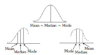
A distribution which is not symmetric is called a skewed-distribution. In a moderately asymmetric
distribution, the interval between the mean and the median is approximately one-third of the interval between the mean and the mode i.e., we have the following empirical relation between them,
Mean – Mode = 3(Mean – Median) Mode = 3 Median – 2 Mean. It is known as Empirical relation.
Illustration-35
The mode of the following distribution is
|
Class interval |
0-10 |
10-20 |
20-30 |
30-40 |
40-50 |
50-60 |
60-70 |
70-80 |
|
Frequency |
5 |
8 |
7 |
12 |
28 |
20 |
10 |
10 |
Solution
Here, maximum frequency is 28. Thus, the class 40-50 is the modal class.
Mode =
= 40+6.666 = 46.67(approx.)
Illustration-36
If in a frequency distribution, the mean and median are 20 and 21 respectively, then its mode is approximately
Solution
mode = 3 median – 2 mean = 3 (21) – 2(20) = 23.
Illustration-37
If in a moderately asymmetrical distribution the mode and the mean of the data are 6 and 9 , respectively, then the median is
Solution
For a moderately skewed distribution,
mode = 3median – 2 mean
6. MEASURES OF DISPERSION
The degree to which numerical data tend to spread about an average value is called the dispersion of the data. The four measure of dispersion are
(1) Range (2) Mean deviation (3) Standard deviation (4) Square deviation
1. RANGE
It is the difference between the values of extreme items in a series. Range =
The coefficient of range (scatter) = .
Range is not the measure of central tendency. Range is widely used in statistical series relating to
quality control in production.
Range is commonly used measures of dispersion in case of changes in interest rates, exchange rate, share prices and like statistical information. It helps us to determine changes in the qualities of the goods produced in factories.
i. Inter-quartile range
We know that quartiles are the magnitudes of the items which divide the distribution into four equal parts. The inter-quartile range is found by taking the difference between third and first quartiles and is given by the following formula,
Inter-quartile range = Q3 – Q1,
where Q1 = First quartile or lower quartile and Q3 = Third quartile or upper quartile.
ii. Percentile range
This is measured by the following formula,
Percentile range = P90 – P10,
where P90 – 90th percentile and P10 = 10th percentile.
Percentile range is considered better than range as well as inter-quartile range.
iii. Quartile deviation or semi inter-quartile range
It is one-half of the difference between the third quartile and first quartile i.e., Q.D. = and coefficient of quartile deviation = , where Q3 is the third or upper quartile and Q1 is the lowest or first quartile.
2. MEAN DEVIATION
The arithmetic average of the deviations (all taking positive) from the mean, median or mode is
known as mean deviation.
Mean deviation is used for calculating dispersion of the series relating to economic and social inequalities. Dispersion in the distribution of income and wealth is measured in term of mean deviation.
i. Mean deviation from ungrouped data (or individual series)
Mean deviation = .
where |x – M| means the modulus of the deviation of the variate from the mean (mean, median or
mode) and n is the number of terms.
ii. Mean deviation from continuous series
Here first of all we find the mean from which deviation is to be taken. Then we find the deviation
dM =|x – M| of each variate from the mean M so obtained.
Next we multiply these deviations by the corresponding frequency and find the product f.dM and then the sum f dM of these products.
Lastly we use the formula, mean deviation =
3. STANDARD DEVIATION
Standard deviation (or S.D.) is the square root of the arithmetic mean of the square of deviations of various values from their arithmetic mean and is generally denoted by s read as sigma. It is used in statistical analysis.
i. Coefficient of standard deviation
To compare the dispersion of two frequency distributions the relative measure of standard deviation is computed which is known as coefficient of standard deviation and is given by
Coefficient of A.D. = , where is the A.M.
ii. Standard deviation from individual series
where, = The arithmetic mean of series
N = The total frequency.
iii. Standard deviation from continuous series
where, = Arithmetic mean of series
xi = Mid value of the class
fi = Frequency of the corresponding
N = Sf = The total frequency
Short cut method
(i) (ii)
where, d = x – A = Deviation from the assumed mean A
f = Frequency of the item
N = f = Sum of frequencies
4. SQUARE DEVIATION
i. Root mean square deviation
where A is any arbitrary number and S is called mean square deviation.
ii. Relation between S.D. and root mean square deviation
If s be the standard deviation and S be the root mean square deviation.
Then, ,
Obviously, S2 will be least when d = 0 i.e.,
Hence, mean square deviation and consequently root mean square deviation is least, if the deviations are taken from the mean.
VARIANCE
The square of standard deviation is called the variance.
Coefficient of standard deviation and variance
The coefficient of standard deviation is the ratio of the S.D. to A.M. i.e., .
Coefficient of variance = coefficient of S.D. .
Variance of the combined series
If are the sizes, the means and the standard deviation of two series, then
where and .
Note :1
if V (X) is variance of X then
V(X + a) = V(X)
V(aX) = a2V(X)
V(aX + b) = a2V(X)
V (aX + bY) = a2v (X) + b2v (Y)
Note :2
For a, a + d, a + 2d, ….., a + (n – 1)d,
Note :3
1) Q.D < M.D < S.D
2)
SKEWNESS
“Skewness” measures the lack of symmetry. It is measured by and is denoted by .
The distribution is skewed if,
(i) Mean Median Mode
(ii) Quartiles are not equidistant from the median
(iii) The frequency curve is stretched more to one side than to the other.
1. Distribution
There are three types of distributions.
(i) Normal distribution :
When , the distribution is said to be normal. In this case, Mean = Median = Mode
(ii) Positively skewed distribution : When , the distribution is said to be positively skewed. In this case, Mean > Median > Mode
(iii) Negative skewed distribution : When , the distribution is said to be negatively skewed. In this case, Mean < Median < Mode
Measures of skewness
(i) Absolute measures of skewness : Various measures of skewness are
(a) (b) (c)
where, Md = median, M0 = mode, M = mean.
Absolute measures of skewness are not useful to compare two series, therefore relative measure of
dispersion are used, as they are pure numbers.
3. Relative measures of skewness
(i) Karl Pearson’s coefficient of skewness
where s is standard deviation.
(ii) Bowley’s coefficient of skewness :
Bowley’s coefficient of skewness lies between –1 and 1.
(iii) Kelly’s coefficient of skewness
Illustration-38
The quartile deviation of daily wages of in (Rs.) of 11 persons given below 140, 145, 130, 165, 160, 125, 150, 170, 175, 120, 180
Solution
The given data in ascending order of magnitude is 120, 125, 130, 140, 145, 150, 160, 165, 170, 175, 180
Here, = 130
Illustration-39
The variance of the first ‘n’ natural numbers is
Solution
Variance
Illustration-40
If the M.D is 12, the value of S.D will be
Solution
We know that
Illustration-41
The mean of five observations is 4 and their variance is 5.2. If three of these observations are 1, 2 and 6, then the other two observations are
Solution
Let the two unknown items be x and y, then
Mean = 4
x + y = 11…..(1) and variance = 5.2
Solving (1) and (2) for x and y, we get
x = 4, y = 7 or x = 7, y = 4.
1. BASICS OF STATISTICS
1. STATISTICAL DATA
Statistical data are the facts which are collected for the purpose of investigation. There are two types of statistical data:
(i) Primary data: The data collected by an investigator for the first time for his own purpose are called primary data. As the primary data are collected by the user of the data, so it is more reliable and relevant.
(ii) Secondary data: The data collected by a secondary source and used by the investigator for his purpose is called secondary data. For example score of a cricket match noted from newspapers is secondary data. Thus data which are primary in the hands of one become secondary in the hands of the other. Data collected by any source also can be divided in following two types:
(i) Raw Data: Raw data are those data which are obtained from the original source but not arranged numerically. This is also called ‘ungrouped data’ for example marks of 10 students in maths are given as: 75, 96, 25, 32, 89, 62, 40, 79, 35, 55 An ‘array’ is an arrangement of raw numerical data in the ascending or descending order of magnitude. Above data can be written as 25, 32, 35, 40, 55, 62, 75, 79, 89, 96
(ii) Grouped data: An array can be placed systematically in groups or categories. For example the above data can be grouped in following manner.
| GROUPS | MARKS | TOTAL NUMBER OF STUDENTS |
| 0 to 20 | – | 0 |
| 21 to 40 | 25, 32, 35, 40 | 4 |
| 41 to 60 | 55 | 1 |
| 61 to 80 | 62, 75, 79 | 3 |
| 81 to 100 | 89, 96 | 2 |
| TOTAL | 10 | |
2. SOME BASIC DEFINITIONS
(i) Variate: Variate is a quantity that may vary from observation to observation.
(ii) Range: Range is difference between the maximum and minimum observations.
(iii) Class Interval: When data are divided in groups, each group is called a class interval.
(iv) Class Limit: Every class interval has two limits. The smallest observation of the interval is called lower limit and the largest observation of the interval is called upper limit.
(v) Class Mark: The mid value of any class is called its class mark.
(vi) Class Size: Class size is defined as the difference between two successive class marks. It is also the difference between the upper and lower limits of any class interval.
(vii) Frequency: In a particular class the count of the number of observation is called its frequency. So the corresponding frequency of a class is called its class frequency.
(viii) Cumulative Frequency: The cumulative frequency of any class is obtained by adding all the frequencies successively prior to that class i.e. it is the sum of all frequencies up to that class.
(ix) True Class Limit: In the case of exclusive classes the upper and lower limits are respectively known as its true upper limits and true lower limits. In the case of inclusive classes, the true lower and upper limits are obtained by subtracting 0.5 from the lower limit and adding 0.5 to the upper limit. True upper limits and true lower limits are also known as boundaries of the class.
(x) Tally: Tally method is used to keep the chance of error at minimum in counting. A bar (|) called tally mark is put against any item when it occurs. The fifth occurrence of any item is represented by putting diagonally a cross tally (\) on the first four tallies.
3. FREQUENCY DISTRIBUTION
The tabular arrangement of data showing the frequency of each item is called a frequency distribution table. It is a method to present raw data in the form from which one can easily understand the information contained in the raw data. Frequency distribution are of two types:
i. Discrete frequency distribution:
In this type of frequency distribution, in the first column of frequency table we write all possible values of the variables from the lowest to the highest, in the second column we write tally marks and in the third column we show frequency of each item. In this method data are not divided into groups or classes.
e.g. no. of girls in 20 families is given in following data:
1, 2, 3, 1, 1, 2, 3, 3, 4, 1, 5, 1, 1, 2, 2, 3, 3, 2, 4, 1
The above data can be put in the form of a discrete frequency distribution table in the following manner:
| S. No. | No. of girls | Tally Marks | Frequency |
| 1. | 1 | 7 | |
| 2. | 2 | 5 | |
| 3. | 3 | 5 | |
| 4. | 4 | || | 2 |
| 5. | 5 | | | 1 |
| TOTAL | 20 | ||
ii. Continuous or Grouped Frequency Distribution
In the frequency distribution data are divided into groups or classes. This method is used only where the values in the raw data are largely repeating and the difference between the greatest and the smallest observations is not very large.
4. CUMULATIVE FREQUENCY
Cumulative frequency table is obtained from the ordinary frequency table by successively adding the several frequencies. Thus to form a cumulative frequency table we add a column of cumulative frequency in the frequency distribution table. It is obvious that the cumulative frequency of the last class is the sum of the frequencies of all the classes.
Cumulative frequency series are of two types:
(i) Less than series (ii) More than series
Illustration -1
The weekly saving of 30 workers working in a factory is as given below:
64, 60, 87, 75, 69, 34, 51, 78, 39, 48, 73, 54, 63, 70, 57, 88, 90, 53, 74, 44, 31, 71, 68, 72, 36, 89, 55, 67, 73, 83
(a) Taking first class interval as 30 – 40 (40 not included), form a frequency table of equal intervals.
(b) Also form a cumulative frequency table.
(c) Find the number of workers whose weekly saving is more than Rs. 60.
Solution
(i) For the given data of the weekly saving of 30 workers working in a factory, we prepare following table:
| S. No. | Class Interval (Saving in Rs.) | Tally Marks | Frequency (No. of workers) |
| 1. | 30 – 40 | | | | | | 4 |
| 2. | 40 – 50 | | | | 2 |
| 3. | 50 – 60 | 5 | |
| 4. | 60 – 70 | 6 | |
| 5. | 70 – 80 | 8 | |
| 6. | 80 – 90 | | | | | | 4 |
| 7. | 90 – 100 | | | 1 |
| TOTAL | 30 |
(ii) For given data cumulative frequency table can be given in the following manner:
| S. No. | Class Interval (Saving in Rs.) | Tally Marks | Frequency (No. of workers) | Cumulative Frequency |
| 1. | 30 – 40 | | | | | | 4 | 4 |
| 2. | 40 – 50 | | | | 2 | 6 |
| 3. | 50 – 60 | 5 | 11 | |
| 4. | 60 – 70 | 6 | 17 | |
| 5. | 70 – 80 | 8 | 25 | |
| 6. | 80 – 90 | | | | | | 4 | 29 |
| 7. | 90 – 100 | | | 1 | 30 |
| TOTAL | 30 |
(iii) Number of workers whose weekly saving is Rs. 60 or more than Rs. 60 = (6 + 8 + 4 + 1) = 19
Illustration -2
Heights of seven persons in cm are 120, 125, 142, 134, 150, 155 and 128. Calculate the range.
Solution
For given data maximum height = 155 cm
and minimum height = 120 cm
Range = maximum height – minimum height
= 155 cm – 120 cm
= 35 cm.
Illustration -3
Form a frequency table from the following table:
| Marks | No. of Students |
| Below 10 | 15 |
| Below 20 | 35 |
| Below 30 | 60 |
| Below 40 | 84 |
| Below 50 | 96 |
| Below 60 | 127 |
| Below 70 | 198 |
| Below 80 | 250 |
Solution
For given data we make classes 0 – 10, 10 – 20, 20 – 30, ….., 70–80.
There are 15 students who obtained below 10 marks, therefore frequency of class 0 – 10 is 15. Again number of students getting below 20 marks is 35.
This includes those students also who obtained below 10 marks.
Number of students who got marks between 10 and 20 i.e. frequency of class
10 – 20 = 35–15 = 20
Thus for given data we make following table:
| S. No. | Class Interval | Comparative | Frequency |
| 1. | 0 – 10 | 15 | 15 |
| 2. | 10 – 20 | 35 | 20 |
| 3. | 20 – 30 | 60 | 25 |
| 4. | 30 – 40 | 84 | 24 |
| 5. | 40 – 50 | 96 | 12 |
| 6. | 50 – 60 | 127 | 31 |
| 7. | 60 – 70 | 198 | 71 |
| 8. | 70 – 80 | 250 | 52 |
| TOTAL | 250 |
Illustration -4
Find the unknown entries (a, b, c, d, e, f, g) from the following frequency distribution of heights of 60 students in a class:
| Height (in cm) | Frequency | Cumulative frequency |
| 160 – 165 | 15 | a |
| 165 – 170 | b | 35 |
| 170 – 175 | 12 | c |
| 175 – 180 | e | 50 |
| 180 – 185 | d | 55 |
| 185 – 190 | 5 | f |
| Total | g |
Solution
From given table, we make following cumulative frequency table:
| S. No. | Height (in cm) | Frequency | Cumulative Frequency |
| 1. | 160 – 165 | 15 | 15 = a |
| 2. | 165 – 170 | b | 15 + b = 35 |
| 3. | 170 – 175 | 12 | 15 + b + 12 = c |
| 4. | 175 – 180 | d | 15 + b + 12 + d = 50 |
| 5. | 180 – 185 | e | 15 + b + 12 + b + e = 55 |
| 6. | 185 – 190 | 5 | 15 + b + 12 + d + e + 5 = f |
| g | 60 |
Now, from table:
a = 15
15 + b = 35 b = 35 – 15 = 20
15 + b + 12 = c 15 + 20 + 12 = c
c = 47
15 + b + 12 + d = 50
15 + 20 + 12 + d = 50
d = 50 – 47
d = 3
15 + b + 12 + d + c = 55
15 + 20 + 12 + 3 + e = 55
e = 55 – 50
e = 5
15 + b + 12 + d + e + 5 = f
15 + 20 + 12 + 3 + 5 + 5 = f
f = 60
g = 60. Hence, a = 15, b = 20, c = 47, d = 3, e = 5, f = 60 and g = 60.
5. GRAPHICAL REPRESENTATION OF DATA
A given data can be represented in graphical way. There are various methods of graphical representation of frequency distribution.
(i) Bar Graphs
(ii) Histogram
(iii) Frequency Polygon
(iv) Pie Chart
Bar Graph
The frequency distribution of a discrete value is best represented by a bar graph. The height of the bars is proportional to the frequency of each variate-value. In a bar graph the bars must be kept distinct to show that the variate-values are distinct. The bars are of equal width and are drawn with equal spacing between them on the x-axis depicting the variable. The values of the variable are shown on the y-axis.
Illustration -5
The following table shows the number of illiterate persons in the age group (10–58 years) in a town:
| Age Group (in years) | 10 – 16 | 17 – 23 | 24 – 30 | 31 – 37 | 38 – 44 | 45 – 51 | 52 – 58 |
| Number of illiterate person | 175 | 375 | 100 | 150 | 250 | 400 | 525 |
Solution
Draw a bar graph to represent the above data.
Histogram
Histogram is a graphical representation of a grouped frequency distribution with continuous classes. It consists of a set of rectangles where heights of rectangles are proportional to their class frequencies, for equal class intervals. There is no gap between two successive rectangles. The rectangles are constructed with base as the class size and their heights representing the frequencies.
Illustration -6
Construct a histogram from the following distribution of total marks obtained by 750 students of class IX in the final examination.
| Marks (mid-points) | 620 | 660 | 700 | 740 | 780 | 820 | 860 |
| Number of students | 16 | 45 | 156 | 284 | 172 | 59 | 18 |
Solution
To draw the histogram for above data first of all we find out class limits for making class intervals from given class marks.
Here difference between second and the first class marks = h = 660 – 620 = 40
lower limit of first class interval = 620 – h/2
= 620 – 20
= 600
And upper limit of the first class interval = = 620 + 20 = 640
Similarly other class intervals would be,
(660 – 20) – (660 + 20), (700 – 20) – (700 + 20), (740 – 20) – (740 + 20), (780 – 20) – (780 + 20), (820 – 20) – (820 + 20) and (860 – 20) – (860 – 20)
i.e. 640 – 680, 680 – 720, 720 – 760, 760 – 800, 800 – 840 and 840 – 880 Using these class intervals we draw following histogram taking class intervals on X-axis and number of students on Y-axis
Frequency Polygon
A frequency polygon is a graph of frequency distribution. It is a line graph of class frequency which is plotted against class mark. A frequency polygon can be obtained by two methods:
(1) By using Histogram: A frequency polygon can be obtained by joining mid points of the top of the rectangles of a histogram. For this we obtain the mid points of the upper horizontal sides of each rectangle and then join these mid points by dotted lines to get frequency polygon. End of a frequency polygon preferably extended to the mid points of imagined class intervals adjacent to first and last class intervals.
Illustration -7
Draw the histogram and frequency polygon of the following frequency distribution:
| Monthly wages (in rupees) | 325-350 | 350-375 | 375-400 | 400-425 | 425-450 | Total |
| Number of workers | 30 | 45 | 75 | 60 | 55 | 245 |
Solution
Using given data we draw histogram taking monthly wages (in rupees) on X-axis and number of workers on Y-axis. Then we join the mid points of the top of the rectangles by dotted straight lines and complete it by joining the mid points of imagined class intervals adjacent to the first and last class intervals.
(2) Frequency polygon without using Histogram: Following procedure is used to make a frequency polygon without using histogram.
(i) Calculate the class marks, x1, x2, …., xn of each of the given class intervals.
(ii) Mark class marks x1, x2, …., xn, along X-axis and frequencies f1, f2, …. fn along Y-axis.
(iii) Plot the points (x1, f1), (x2, f2), ,….., (xn, fn).
(iv) Obtain the mid-points of two class intervals of zero frequencies at the beginning of the first interval and at the end of the last interval.
(v) Join the points (x1, f1), (x2, f2), …, (xn, fn) by the line segments and complete the frequency polygon by joining the mid points of the first and last intervals to the mid points of the imagined classes adjacent to them.
Illustration -8
Represent the following distribution by a frequency polygon without using a histogram:
| Scores | 20-29 | 30-39 | 40-49 | 50-59 | 60-69 | 70-79 | 80-89 | 90-99 |
| Frequency | 2 | 5 | 3 | 18 | 20 | 22 | 12 | 7 |
Solution
Given data is in the form of inclusive classes, so first of all we shall convert them into exclusive classes. Also we have to get class marks of these class intervals for this purpose.
| S. No. | Scores | True Class Limits | Class Marks | Frequency | Points to be plotted |
| 1. | 20 – 29 | 19.5 – 29.5 | 24.5 | 2 | (24.5, 2) |
| 2. | 30 – 39 | 29.5 – 39.5 | 34.5 | 5 | (34.5, 5) |
| 3. | 40 – 49 | 39.5 – 49.5 | 44.5 | 3 | (44.5, 3) |
| 4. | 50 – 59 | 49.5 – 59.5 | 54.5 | 18 | (54.5, 18) |
| 5. | 60 – 69 | 59.5 – 69.5 | 64.5 | 20 | (64.5, 20) |
| 6. | 70 – 79 | 69.5 – 79.5 | 74.5 | 22 | (74.5, 22) |
| 7. | 80 – 89 | 79.5 – 89.5 | 84.5 | 12 | (84.5, 12) |
| 8. | 90 – 99 | 89.5 – 99.5 | 94.5 | 7 | (94.5, 7) |
Plotting these points and joining them by line segments we get frequency polygon. We complete the frequency polygon by extending it up to points (14.5, 0) and (104.5, 0) adjacent to first and last class marks on X-axis.
Pie Chart
In a pie-chart, various observations or components are represented by the sectors of a circle and the whole circle represents the sum of the values of all the components. Clearly, the total angle of 360o at the center of the circle is divided according to the values of the components. Thus we have, Central Angle for Component
=
Sometimes, the value of components are expressed in percentages. In such cases, we have: Central Angle for Component =
Illustration -9
A survey was conducted among a group of girls to know their preferences for the types of slippers. The given circle graph shows the results of the survey.
If the survey was conducted among a group of 1080 girls, then find out how many girls preferred to wear leather slippers?
(A) 140 (B) 280 (C) 420 (D) 560
Solution
C
In the given circle graph, it is seen that the central angle of the sector corresponding to leather slippers is 140°.
Therefore, number of girls who preferred to wear leather slippers:
Thus, 420 girls preferred to wear leather slippers.
6. MEASURES OF CENTRAL TENDENCY
One of the most important objectives of statistical analysis is to get one single value that describes the characteristic of the entire data. Such a value is called the central value or an average. The following are the important types of averages:
1. Arithmetic Mean
2. Geometric Mean
3. Harmonic mean
4. Median
5. Mode
We consider these measures in three cases (i) Individual series (i.e. each individual observation is given) (ii) discrete series (i.e., the observations along with number of times a particular observation called the frequency is given) (iii) continuous series (i.e. the class intervals along with their frequencies are given)
2. Arithmetic Mean
The average of numbers in arithmetic is known as the Arithmetic Mean of these numbers in statistics.
1. MEAN OF AN UNGROUPED DATA
The Arithmetic Mean or simply the Mean of n observations x1, x2, x3, …….xn is given by the formula:
Mean =
Where the symbol , called sigma stands for the summation of the terms.
Illustration -10
Calculate the mean of the following numbers: 3, 1, 5, 6, 3, 4, 5, 3, 7, 2
Solution
Sum of the given numbers = (3 + 1 + 5 + 6 + 3 + 4 + 5 + 3 + 7 + 2) = 39.
Number of these numbers = 10.
Mean of the given numbers = .
Illustration -11
The weights (in kg) of 5 persons in a group are: 55, 63, 48, 59 and 61. Find their mean weight.
Solution
Sum of the weight of all persons = (55 + 63 + 48 + 59 + 61) kg = 286 kg.
Number of persons = 5.
Mean weight = kg = 57.2 kg.
Some Useful Result: Let the mean of x1 x2 x3, ……..xn be A. Then
(i) Mean of (x1 + k), (x2 + k), (x3+ k) ………..(xn + k) is (A + k);
(ii) Mean of (x1 – k), (x2 – k), (x3 – k)………..(xn – k) is (A – k);
(iii) Mean of kx1, kx2, kx3 …….. kxn is kA, where k 0.
2. MEAN OF GROUPED DATA
Direct Method
When the variates x1, x2, x3, …………xn have frequencies f1, f2, f3 ……..fn respectively, then the mean is given by the formula:
Mean = .
Illustration -12
The following table shows the weights of 15 members of an athletic team in a school.
| Weight (in kg) | 42 | 45 | 46 | 48 | 49 |
| Number of athletes | 4 | 3 | 5 | 2 | 1 |
Find the mean weight.
Solution
From the above data, we may prepare the table given below.
|
Weight (in kg) xi |
Number of athletes (Frequency) |
|
|
42 45 46 48 49 |
4 3 5 2 1 |
168 135 230 96 49 |
|
|
= 15 |
= 678 |
Mean Weight =.
Illustration -13
Using short cut method, calculate the mean weekly wage from the following frequency distribution.
| Weekly wages(in Rs) | 950 | 1000 | 1050 | 1100 | 1250 | 1500 | 1600 |
| Number of workers | 24 | 18 | 13 | 15 | 20 | 11 | 9 |
Solution
Let the assumed mean be, A = 1100.
From the given data, we may prepare the table given below.
|
Weekly Wages (in Rs) x1 |
Numbers of Workers (Frequency) |
di = (xi – A) = (xi – 1100) |
fidi |
|
950 1000 1050 1100 = A 1250 1500 1600 |
24 18 13 15 20 11 9 |
–150 –100 –50 0 150 400 500 |
–3600 –1800 –650 0 3000 4400 4500 |
|
|
fI = 110 |
|
fI di = 5850 |
Mean =
Hence, Mean Wage = Rs 1153.18.
3. MEAN OF GROUPED DATA IN THE FORM OF CLASSES
I. Direct Method
Step 1: For each class, find the class mark xi by using the relation, xi = (lower limit + upper limit). Step 2: Use the formula, Mean = .
II. Short Cut Method or Deviation Method
Step 1: For each class, find the class mark xi.
Step 2: Let A be the assumed mean.
Step 3: Find di = (xi – A).
Step 4: Use the formula, Mean = .
III. Step-Deviation Method
Step 1. For each class, find the class mark x1.
Step 2: Let A be the assumed mean.
Step 3: Calculate, , where c is the class size.
Step 4: Use the formula, Mean = .
Illustration -14
Using direct method, find the mean of the following frequency distribution:
| Class-interval | 10-20 | 20-30 | 30-40 | 40-50 | 50-60 | 60-70 |
| Frequency | 6 | 8 | 12 | 15 | 10 | 9 |
Solution
From the given data, we may prepare the table given below.
|
Class-Interval |
Class-Mark xi |
Frequency fi |
fixi |
|
10-20 20-30 30-40 40-50 50-60 60-70 |
15 25 35 45 55 65 |
6 8 12 15 10 9 |
90 200 420 675 550 585 |
|
|
|
fI = 60 |
fixi = 2520 |
Mean = .
Illustration -15
Using Short Cut Method find the mean for the following frequency distribution:
| Class-interval | 84-90 | 90-96 | 96-102 | 102-108 | 108-114 | 114-120 |
| Frequency | 8 | 10 | 16 | 23 | 12 | 11 |
Solution
From the given data, we may prepare the table given below.
|
Class-Interval |
Class-Mark xi |
Frequency fi |
di = (xi – A) = (xi – 99) |
fidi |
|
84-90 90-96 96-102 102-108 108-114 114-120 |
87 93 99 = A 105 111 117 |
8 10 16 23 12 11 |
–12 –6 0 6 12 18 |
–96 –60 0 138 144 198 |
|
|
|
fI = 80 |
|
fidi = 324 |
Mean =
Hence, Mean = 103.05.
Illustration -16
Using Step Deviation Method, calculate the mean for the following data:
| Height (in cm) | 135-140 | 140-145 | 145-150 | 150-155 | 155-160 | 160-165 | 165-170 | 170-175 |
| Frequency | 4 | 9 | 18 | 28 | 24 | 10 | 5 | 2 |
Solution
Here, class size, c = 5. Take assumed mean, A = 152.5. Thus, from the given data, we may prepare
|
Class-Interval |
Class-Mark xi |
Frequency fi |
fii |
|
|
135-140 140-145 145-150 150-155 155-160 160-165 165-170 170-175- |
137.5 142.5 147.5 152.5 = A 157.5 162.5 167.5 172.5 |
4 9 18 28 24 10 5 2 |
–3 –2 –1 0 1 2 3 4 |
–12 –18 –18 0 24 20 15 8 |
|
|
|
fI = 100 |
|
fii = 19 |
Mean = = (152.5 + 0.95) = 153.45 cm.
4. IMPORTANT FORMULAE FOR SOLVING ARITHMETIC MEAN
1. Arithmetic Mean of Individual Series
If x1, x2 , x3,….., xn are n values of variant x, then its Arithmetic Mean, denoted by x is
(or)
where A is the assumed average. (For individual series)
2. Arithmetic Mean of Discreate Series
If a variable takes values x1, x2 , x3,….., xn with corresponding frequencies f1, f2 , f3,….., fn then the arithmetic mean is given by
where
3. Arithmetic Mean Of Continuous Series
In case of a set of data with class intervals, we cannot find the exact value of the mean because we do not know the exact values of the variables. We, therefore, try to obtain an approximate value of the mean. The method of approximate is to replace all the observed values belonging to a class by mid-value of the class.
If x1, x2 , x3,….., xn are the mid values of the class intervals having corresponding frequencies f1, f2 , f3,….., fn then we apply the same formula as in discrete series.
4. Combined Arithmetic Mean
If are the means of k – series of sizes then the combined or composite mean can be obtained by the formula :
5. Weighted Arithmetic Mean
If w1, w2 , w3,….., wn be the weights assigned to the values x1, x2 , x3,….., xn be respectively of a variable x, then the weighted A.M. is .
5. PROPERTIES OF ARITHMETIC MEAN
1. Sum of all the deviations from arithmetic mean is zero i.e.,
(in case of individual series)
(in case of discrete or continuous series)
2. If each observation is increased or decreased by a given constant K, the mean is also increased or decreased by K
The property is also known as effect of change of origin. K can be taken to be any number. However, to simplify the calculations, K should be taken as a value which is in the middle of the table.
3. Step Deviation Method or change of scale
If x1, x2 , x3,….., xn are mid values of class intervals with corresponding frequencies f1, f2 , f3,….., fn then we may change the scale by taking in this case.
(if A is assumed mean)
A and h can be any numbers but if the lengths of class intervals are equal then h may be taken as width of the class interval.
In particular if each observation is multiplied or divided by a constant, the mean is also multiplied or divided by the same constant.
4. The sum of the squared deviation of the variate from their mean is minimum i.e., the quantity is minimum when .
5. E(aX + b) = aE(X) + b (where E(X) = Mean of X)
Illustration-17
The weighted mean of the first n natural numbers, the weights being the corresponding numbers, is
Solution
First n natural numbers are 1, 2, 3,…,n; whose corresponding weights are 1, 2, 3,…,n respectively.
weight mean =
Illustration-18
The weighted mean of the first n natural numbers whose weights are equal to the squares of the corresponding numbers is
Solution
weighted mean =
Illustration-19
The average salary of male employees in a firm is Rs. 5200 and that of females is Rs.4200. The mean salary of all the employees is Rs.5000. The percentage of male and female employees are respectively is
Solution
Let
Also, we know that
The percentage of male employees in the firm =
and the percentage of female employees in the firm =
Illustration-20
If the mean of 9 observations is 100 and mean of 6 observations is 80, then the mean of 15 observations is
Solution
Illustration-21
If a variate X is expressed as a linear function of two variates U and V in the form X = aU + bV then the mean of X is
Solution
We have
Illustration-22
If the arithmetic mean of the numbers x1, x2 , x3,….., xn is , then the arithmetic mean of the numbers , where a, b are two constants, would be
Solution
Required mean
Illustration-23
If the mean of the numbers 27+x, 31+x, 89+x , 107+x, 156+x is 82, then the mean of 130+x, 126+x, 68+x, 50+x, 1+x is
Solution
Given
Therefore, the required mean is
Illustration-24
A student obtain 75%, 80% and 85% in three subjects. If the marks of another subject is added, then his average cannot be less than
Solution
Marks obtained from three subjects out of 300 is 75+80+85 = 240
If the marks of another subject is added, then the marks will be 240 out of 400
minimum average marks =
[when marks in the fourth subject = 0]
Illustration-25
The mean of 100 items is 49. It was discovered that three items which should have been 60, 70, 80 were wrongly read as 40, 20, 50 respectively. The correct mean is
Solution
Sum of 100 items = 49 × 100 = 4900
sum of items added = 60+ 70+80=210
new sum = 4900+210–110=5000
correct mean =
Illustration-26
The mean weight per student in a group of seven students is 55kg. If the individual weights of six students are 52, 58, 55, 53, 56 and 54, then the weight of the seventh student is
Solution
The total weight of seven students is 55×7 = 385kg
The sum of the weights of six students is 52+58+55+53+56+54 = 328kg
Hence, the weight of the seventh student is = 385 – 328 = 57kg
3. GEOMETRIC MEAN
1. GEOMETRIC MEAN IN INDIVIDUAL SERIES
1. If x1, x2 , x3,….., xn are n values of a variate x, none of them being zero, then geometric mean (G.M.) is given by G.M =
2. log (G.M.) =
2. GEOMETRIC MEAN IN DISCRETE SERIES
In case of frequency distribution, G.M. of n values x1, x2 , x3,….., xn of a variate x occurring with frequency f1, f2 , f3,….., fn is given by G.M = , where .
Illustration-27
The geometric mean of the numbers is
Solution
Illustration-28
Find the geometric mean of the following values:
Solution
Given data, 15, 12, 13, 19, 10
|
X |
Log x |
|
15 |
1.1761 |
|
12 |
1.0792 |
|
13 |
1.1139 |
|
19 |
1.2788 |
|
10 |
1.0000 |
|
Total |
5.648 |
log x =5.648 and n = 5
log(G.M.) = .
= Antilog
= Antilog 1.1296
= 13.48
Answer: Geometric Mean = 13.48
4. HARMONIC MEAN
The harmonic mean is based on the reciprocals of the value of the variable
(Incase of Individual series) and (in case of discrete series or continuous series)
Relation among Arithmetic Mean, Geometric Mean and Harmonic Mean
The Arithmetic Mean (A. M.), Geometric Mean (G.M.) and Harmonic Mean (H.M.) for a given set of observations x1, x2 , x3,….., xn > 0 of a series are related as under:
Illustration-29
The harmonic mean of 3, 7, 8, 10, 14 is
(A) (B) (C) (D)
Solution
D
H.M. =
Illustration-30
Find the harmonic mean of , occurring with frequencies 1, 2, 3,…..n, respectively.
Solution
We know that, Harmonic mean =
and
Which is an arithmetic progression with a = 2 and d = 1.
By the formula of sum of n term of an A.P,
we have =
Harmonic mean
5. MEDIAN AND MODE
1. MEDIAN
The median is the central value of the set of observations provided all the observations are arranged in the ascending or descending orders. It is generally used, when effect of extreme items is to be kept out.
Calculation of median
(i) Individual series: If the data is raw, arrange in ascending or descending order. Let n be the number of observations.
If n is odd, Median = value of item.
If n is even, Median =
(ii) Discrete series : In this case, we first find the cumulative frequencies of the variables arranged in ascending or descending order and the median is given by Median = observation, where n is the cumulative frequency.
(iii) For grouped or continuous distributions : In this case, following formula can be used.
(a) For series in ascending order, Median =
Where
l = Lower limit of the median class
f = Frequency of the median class
N = The sum of all frequencies
i = The width of the median class
C = The cumulative frequency of the class preceding to median class.
(b) For series in descending order
Median = , where u = upper limit of the median class,
As median divides a distribution into two equal parts, similarly the quartiles, quantiles, deciles and percentiles divide the distribution respectively into 4, 5, 10 and 100 equal parts. The jth quartile is given by . Q1 is the lower quartile, Q2 is the median and Q3 is called the upper quartile.
(2) Lower quartile
(i) Discrete series :
(ii) Continuous series :
(3) Upper quartile
(i) Discrete series :
(ii) Continuous series :
(4) Decile : Decile divide total frequencies N into ten equal parts.
, [where j = 1, 2, 3, 4, 5, 6, 7, 8, 9]
If j = 5, then . Hence D5 is also known as median.
(5) Percentile : Percentile divide total frequencies N into hundred equal parts and , where k = 1, 2, 3, 4, 5,…….,99.
Illustration-31
The median of 10, 14, 11, 9, 8, 12, 6 is
(A) 10 (B) 12 (C) 14 (D) 11
Solution
(A)
Arrange the items in ascending order i.e., 6, 8, 9, 10, 11, 12, 14.
If n is odd then, Median = value of term
Median = term = 4th term = 10.
Illustration-32
The median of a set of nine distinct observations is 20.5. If each of the last four observations of the set is increased by 2, then the median of the new set is
Solution
Since n = 9, median term = = 5th term.
Now, the last four observations are increased by 2. Since the median is the 5th observation, which remains unchanged, there will be no change in median.
Illustration-33
If a variable takes the discrete value then the median is
Solution
Arrange the data as follows:
median = [value of 4th item+value of 5th item]
median =
Illustration-34
The median of distribution 83, 54, 78, 64, 90, 59, 67, 72, 70, 73 is
Solution
On arranging in ascending order, we get 54, 59, 64, 67, 70, 72, 73, 78, 83, 90
n = 10
=
2. MODE
The mode or model value of a distribution is that value of the variable for which the frequency is maximum. For continuous series, mode is calculated as,
Mode =
Where, l1 = The lower limit of the model class
f1 = The frequency of the model class
f0 = The frequency of the class preceding the model class
f2 = The frequency of the class succeeding the model class
i = The size of the model class.
Symmetric distribution
A distribution is a symmetric distribution if the values of mean, mode and median coincide. In a
symmetric distribution frequencies are symmetrically distributed on both sides of the centre point of the frequency curve.
A distribution which is not symmetric is called a skewed-distribution. In a moderately asymmetric
distribution, the interval between the mean and the median is approximately one-third of the interval between the mean and the mode i.e., we have the following empirical relation between them,
Mean – Mode = 3(Mean – Median) Mode = 3 Median – 2 Mean. It is known as Empirical relation.
Illustration-35
The mode of the following distribution is
|
Class interval |
0-10 |
10-20 |
20-30 |
30-40 |
40-50 |
50-60 |
60-70 |
70-80 |
|
Frequency |
5 |
8 |
7 |
12 |
28 |
20 |
10 |
10 |
Solution
Here, maximum frequency is 28. Thus, the class 40-50 is the modal class.
Mode =
= 40+6.666 = 46.67(approx.)
Illustration-36
If in a frequency distribution, the mean and median are 20 and 21 respectively, then its mode is approximately
Solution
mode = 3 median – 2 mean = 3 (21) – 2(20) = 23.
Illustration-37
If in a moderately asymmetrical distribution the mode and the mean of the data are 6 and 9 , respectively, then the median is
Solution
For a moderately skewed distribution,
mode = 3median – 2 mean
6. MEASURES OF DISPERSION
The degree to which numerical data tend to spread about an average value is called the dispersion of the data. The four measure of dispersion are
(1) Range (2) Mean deviation (3) Standard deviation (4) Square deviation
1. RANGE
It is the difference between the values of extreme items in a series. Range =
The coefficient of range (scatter) = .
Range is not the measure of central tendency. Range is widely used in statistical series relating to
quality control in production.
Range is commonly used measures of dispersion in case of changes in interest rates, exchange rate, share prices and like statistical information. It helps us to determine changes in the qualities of the goods produced in factories.
i. Inter-quartile range
We know that quartiles are the magnitudes of the items which divide the distribution into four equal parts. The inter-quartile range is found by taking the difference between third and first quartiles and is given by the following formula,
Inter-quartile range = Q3 – Q1,
where Q1 = First quartile or lower quartile and Q3 = Third quartile or upper quartile.
ii. Percentile range
This is measured by the following formula,
Percentile range = P90 – P10,
where P90 – 90th percentile and P10 = 10th percentile.
Percentile range is considered better than range as well as inter-quartile range.
iii. Quartile deviation or semi inter-quartile range
It is one-half of the difference between the third quartile and first quartile i.e., Q.D. = and coefficient of quartile deviation = , where Q3 is the third or upper quartile and Q1 is the lowest or first quartile.
2. MEAN DEVIATION
The arithmetic average of the deviations (all taking positive) from the mean, median or mode is
known as mean deviation.
Mean deviation is used for calculating dispersion of the series relating to economic and social inequalities. Dispersion in the distribution of income and wealth is measured in term of mean deviation.
i. Mean deviation from ungrouped data (or individual series)
Mean deviation = .
where |x – M| means the modulus of the deviation of the variate from the mean (mean, median or
mode) and n is the number of terms.
ii. Mean deviation from continuous series
Here first of all we find the mean from which deviation is to be taken. Then we find the deviation
dM =|x – M| of each variate from the mean M so obtained.
Next we multiply these deviations by the corresponding frequency and find the product f.dM and then the sum f dM of these products.
Lastly we use the formula, mean deviation =
3. STANDARD DEVIATION
Standard deviation (or S.D.) is the square root of the arithmetic mean of the square of deviations of various values from their arithmetic mean and is generally denoted by s read as sigma. It is used in statistical analysis.
i. Coefficient of standard deviation
To compare the dispersion of two frequency distributions the relative measure of standard deviation is computed which is known as coefficient of standard deviation and is given by
Coefficient of A.D. = , where is the A.M.
ii. Standard deviation from individual series
where, = The arithmetic mean of series
N = The total frequency.
iii. Standard deviation from continuous series
where, = Arithmetic mean of series
xi = Mid value of the class
fi = Frequency of the corresponding
N = Sf = The total frequency
Short cut method
(i) (ii)
where, d = x – A = Deviation from the assumed mean A
f = Frequency of the item
N = f = Sum of frequencies
4. SQUARE DEVIATION
i. Root mean square deviation
where A is any arbitrary number and S is called mean square deviation.
ii. Relation between S.D. and root mean square deviation
If s be the standard deviation and S be the root mean square deviation.
Then, ,
Obviously, S2 will be least when d = 0 i.e.,
Hence, mean square deviation and consequently root mean square deviation is least, if the deviations are taken from the mean.
VARIANCE
The square of standard deviation is called the variance.
Coefficient of standard deviation and variance
The coefficient of standard deviation is the ratio of the S.D. to A.M. i.e., .
Coefficient of variance = coefficient of S.D. .
Variance of the combined series
If are the sizes, the means and the standard deviation of two series, then
where and .
Note :1
if V (X) is variance of X then
V(X + a) = V(X)
V(aX) = a2V(X)
V(aX + b) = a2V(X)
V (aX + bY) = a2v (X) + b2v (Y)
Note :2
For a, a + d, a + 2d, ….., a + (n – 1)d,
Note :3
1) Q.D < M.D < S.D
2)
SKEWNESS
“Skewness” measures the lack of symmetry. It is measured by and is denoted by .
The distribution is skewed if,
(i) Mean Median Mode
(ii) Quartiles are not equidistant from the median
(iii) The frequency curve is stretched more to one side than to the other.
1. Distribution
There are three types of distributions.
(i) Normal distribution :
When , the distribution is said to be normal. In this case, Mean = Median = Mode
(ii) Positively skewed distribution : When , the distribution is said to be positively skewed. In this case, Mean > Median > Mode
(iii) Negative skewed distribution : When , the distribution is said to be negatively skewed. In this case, Mean < Median < Mode
Measures of skewness
(i) Absolute measures of skewness : Various measures of skewness are
(a) (b) (c)
where, Md = median, M0 = mode, M = mean.
Absolute measures of skewness are not useful to compare two series, therefore relative measure of
dispersion are used, as they are pure numbers.
3. Relative measures of skewness
(i) Karl Pearson’s coefficient of skewness
where s is standard deviation.
(ii) Bowley’s coefficient of skewness :
Bowley’s coefficient of skewness lies between –1 and 1.
(iii) Kelly’s coefficient of skewness
Illustration-38
The quartile deviation of daily wages of in (Rs.) of 11 persons given below 140, 145, 130, 165, 160, 125, 150, 170, 175, 120, 180
Solution
The given data in ascending order of magnitude is 120, 125, 130, 140, 145, 150, 160, 165, 170, 175, 180
Here, = 130
Illustration-39
The variance of the first ‘n’ natural numbers is
Solution
Variance
Illustration-40
If the M.D is 12, the value of S.D will be
Solution
We know that
Illustration-41
The mean of five observations is 4 and their variance is 5.2. If three of these observations are 1, 2 and 6, then the other two observations are
Solution
Let the two unknown items be x and y, then
Mean = 4
x + y = 11…..(1) and variance = 5.2
Solving (1) and (2) for x and y, we get
x = 4, y = 7 or x = 7, y = 4.